Tokenization converts text into the discrete symbols a language model was trained to consume. Its design controls which patterns get their own symbols, how many sequence positions a document uses, and how the model’s embedding rows are addressed. A tokenizer does not add knowledge by itself: a medical vocabulary can encode medical text efficiently without understanding a diagnosis.
We will follow text into token IDs, build a small BPE tokenizer by hand, then use that mechanism to reason about bytes, other subword algorithms, and domain-specific evaluation. The examples start small enough to audit on paper. The later experiments distinguish a synthetic domain comparison, a real held-out vocabulary sweep, and illustrative cost arithmetic.
From a string to a model input
Consider one sentence:
The cat chased the mouse.A conventional Transformer language model accepts numeric tensors. Computers can store strings, and models can be designed to operate on characters or bytes; the narrower point is that this model’s input interface expects a sequence of discrete integer identifiers. The tokenizer supplies that interface.
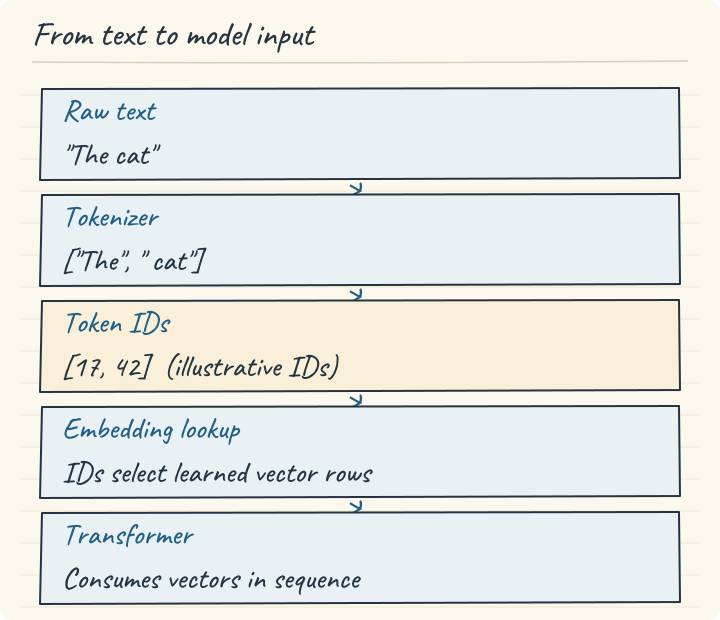
A token is a piece of text; its ID is a vocabulary index. The model receives vectors selected by those IDs.
Suppose we choose a deliberately simple word-and-punctuation tokenizer. It might produce:
pieces: ["The", "cat", "chased", "the", "mouse", "."]
IDs:    [   7,     3,        9,     4,       8,   2]
These IDs are invented for this example. They are not the output of an OpenAI, Llama, or BERT tokenizer. The distinction matters because there is no universal numeric ID for the string cat.
| Term | Meaning in this example |
|---|---|
| Token | One unit selected by the tokenizer, such as |
| Token ID | The vocabulary index assigned to that unit, such as |
| Vocabulary | The mapping between supported units and IDs |
| Embedding | The learned vector retrieved from the model’s embedding table using an ID |
An embedding lookup might use E[3] to fetch the vector associated with cat. If the embedding table has shape , then is the number of vocabulary rows and is the vector width. Six IDs retrieve six rows, yielding a input representation. Attention operates on these vectors later; it does not choose the token boundaries.
IDs are addresses, not measures of meaning. An ID of 9 is not more semantic, more important, or three times the meaning of ID 3. The vocabulary assignment and learned model parameters define the relationship.
The tokenizer is a pipeline
It is tempting to equate the tokenizer with its subword algorithm. A deployed tokenizer also has decisions around that algorithm:
- Normalization: whether text is lowercased, accent-stripped, or Unicode-normalized.
- Pre-tokenization: which spans may be segmented together, such as words, whitespace runs, or digit groups.
- Segmentation: word lookup, BPE, WordPiece, Unigram, or another method.
- Post-processing: optional special tokens and sequence templates.
- Decoding: how pieces reconstruct a string.
For example, BPE restricted to word spans cannot merge across a space, regardless of how frequently that space-separated phrase occurs. Two tokenizers can use BPE and still produce different results because they normalize differently, use different boundaries, or learned different merges. Hugging Face’s pipeline documentation distinguishes these stages.
Normalization is also a preservation decision. Lowercasing The into the loses original case unless another mechanism records it. A tokenizer can faithfully decode its normalized input while being unable to recover the original string. Exact round-trip behavior must be tested for the full pipeline, not assumed from the algorithm name.
Choosing the size of a token
There are three useful starting points. The following segmentations are schematic designs for the same sentence, not measurements from a named model:
word:      The | cat | chased | the | mouse | .
character: T | h | e | ␠ | c | a | t | ␠ | c | h | a | s | e | d | ...
subword:   The | ␠cat | ␠chas | ed | ␠the | ␠mouse | .
Here ␠ makes an ordinary space visible. It is a notation for the diagram, not a claim that the tokenizer literally emits that character.
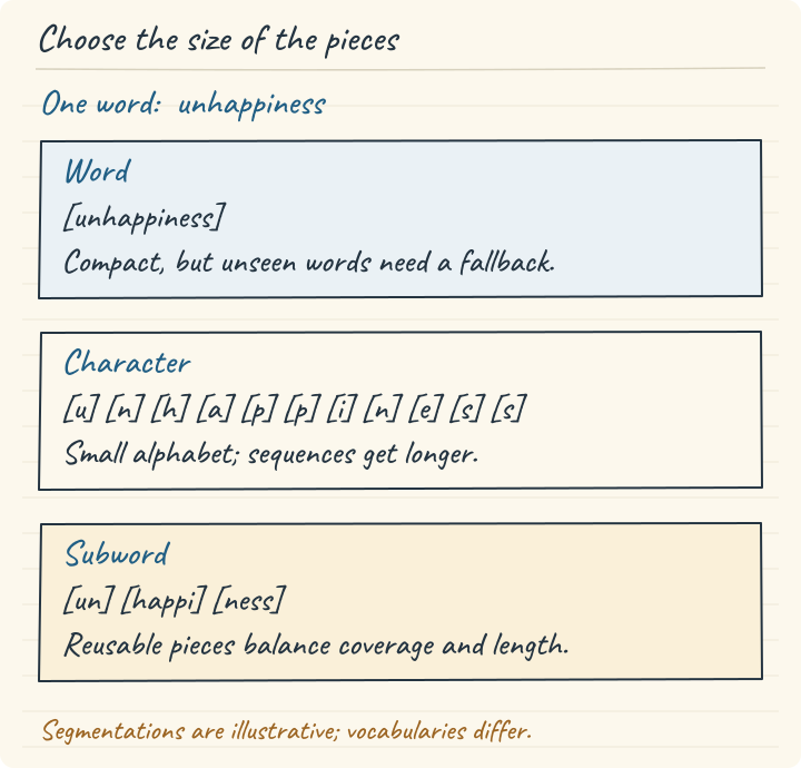
Granularity changes both the size of the vocabulary and the number of positions the model must process.
Word tokens are easy for humans to interpret. If mouse appears often, assigning it one position is economical. But a word vocabulary has to choose what counts as a word, whether to include punctuation, and how to handle inflections, names, compounds, typos, and new terminology. Natural text keeps introducing forms such as mouse, mice, mouselike, and previously unseen identifiers.
A fixed word vocabulary eventually sees a string it does not contain. This is the out-of-vocabulary, or OOV, problem. Replacing every unfamiliar word with [UNK] makes unrelated strings share the same model input. Adding every possible word is not practical, particularly across languages with rich morphology or writing systems without space-delimited words.
Character tokenization reduces this pressure. An unseen word can be represented using familiar characters. However, it only covers characters in its base alphabet unless it has a fallback. Training on English characters does not automatically make it cover every script, combining mark, or emoji.
A minimal character tokenizer makes the mapping explicit. Sorting the alphabet gives reproducible IDs; it does not give those IDs semantic significance.
training_text = "The cat chased the mouse."
alphabet = sorted(set(training_text))
character_to_id = {character: index for index, character in enumerate(alphabet)}
ids = [character_to_id[character] for character in training_text]
decoded = "".join(alphabet[index] for index in ids)
assert decoded == training_text
print(len(training_text), len(ids), len(alphabet))
print(decoded)
Executed output:
25 25 13
The cat chased the mouse.
Characters also produce long sequences. A frequent technical term of twenty characters consumes twenty positions, even if it appears in thousands of documents. A model can learn relations between those positions, but it has to spend sequence capacity reconstructing patterns the tokenizer could have represented more compactly.
Subword tokenization keeps a reusable base while learning larger recurring pieces. A common whole word may become one token. A rarer word may share a stem or suffix with other words. A new word can fall back to smaller pieces. The aim is a useful compromise between a huge word inventory and a long character sequence.
“Subword” does not guarantee linguistically meaningful morphemes. A learned piece might be a suffix, half a syllable, a punctuation pattern, or a byte sequence spanning a boundary permitted by the pre-tokenizer. Frequency and the training objective determine it.
Counting the evidence for a BPE merge
Byte Pair Encoding, adapted to subword learning in Sennrich, Haddow, and Birch, starts with small units and repeatedly combines adjacent units. We will first use characters. Despite its name, this educational BPE example does not yet use raw bytes.
Our training corpus is represented as a frequency dictionary:
| Word | Occurrences |
|---|---|
low | 5 |
lower | 2 |
newest | 6 |
widest | 3 |
This means sixteen word occurrences, not four equally weighted observations. newest: 6 stands for six occurrences of newest. Keeping the string once with its count avoids storing duplicates without discarding their statistical weight.
For this toy tokenizer, pre-tokenization has already separated words. Append the special boundary symbol </w> to each word:
low:     l | o | w | </w>                 × 5
lower:   l | o | w | e | r | </w>         × 2
newest:  n | e | w | e | s | t | </w>     × 6
widest:  w | i | d | e | s | t | </w>     × 3
The boundary is one atomic symbol here, not the four literal characters <, /, w, >. This convention lets a piece distinguish a word-ending occurrence from an internal occurrence. Modern tokenizer implementations use different boundary designs; </w> is not a universal BPE requirement.
In newest, the adjacent pairs are:
(n,e) (e,w) (w,e) (e,s) (s,t) (t,</w>)Each pair occurs once in that spelling and the spelling occurs six times. Therefore each pair contributes six to the corpus pair count. Now inspect widest. It also contains (e,s), (s,t), and (t,</w>), contributing three to each.
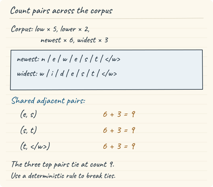
Word frequencies weight every adjacent-pair occurrence. A tie is real; selecting e + s first is a stated tie-break choice.
The resulting shared counts are:
The count is not “two words contain the pair.” It is “nine weighted occurrences contain this adjacency.” Counting only the distinct spellings would change the learned tokenizer.
The general rule is:
is the set of distinct training words, is a word’s corpus frequency, is its current symbol sequence, and counts adjacent occurrences of pair in that sequence. “Current” matters because the sequence changes after every merge.
If abab occurs nine times, (a,b) appears twice in each occurrence:
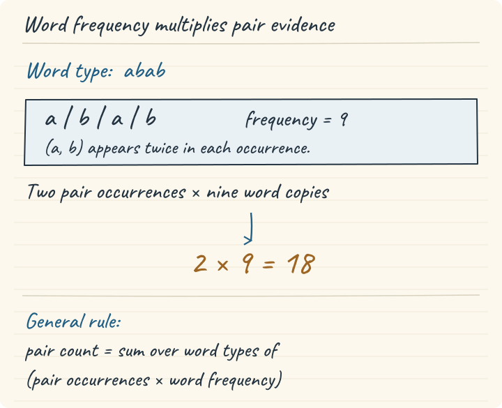
A frequency dictionary compresses repeated strings without discarding their contribution to pair counts.
There is a second edge case. In aaaa, (a,a) occurs at three adjacent positions, so nine copies contribute to pair counting. But a left-to-right non-overlapping replacement can merge only two pairs in each occurrence: aa | aa. Counting candidate positions and applying disjoint replacements are different operations. A toy implementation should make that convention explicit.
Here is the complete initial pair table for our four spellings:
| Pair | Weighted count | Contribution |
|---|---|---|
e + s | 9 | 6 from newest, 3 from widest |
s + t | 9 | 6 + 3 |
t + </w> | 9 | 6 + 3 |
w + e | 8 | 2 from lower, 6 from newest |
l + o | 7 | 5 from low, 2 from lower |
o + w | 7 | 5 + 2 |
e + w | 6 | newest |
n + e | 6 | newest |
w + </w> | 5 | low |
d + e, i + d, w + i | 3 each | widest |
e + r, r + </w> | 2 each | lower |
The small table already shows the connection to domain specialization. Repetition gives particular adjacencies more weight. A medical corpus changes that evidence distribution; it does not change BPE into a medical reasoning system.
Learning BPE one state at a time
Choose the most frequent pair, combine its two symbols into one new symbol, replace its occurrences, and count again. Stop at a merge budget, a target vocabulary limit, or when no eligible pairs remain.
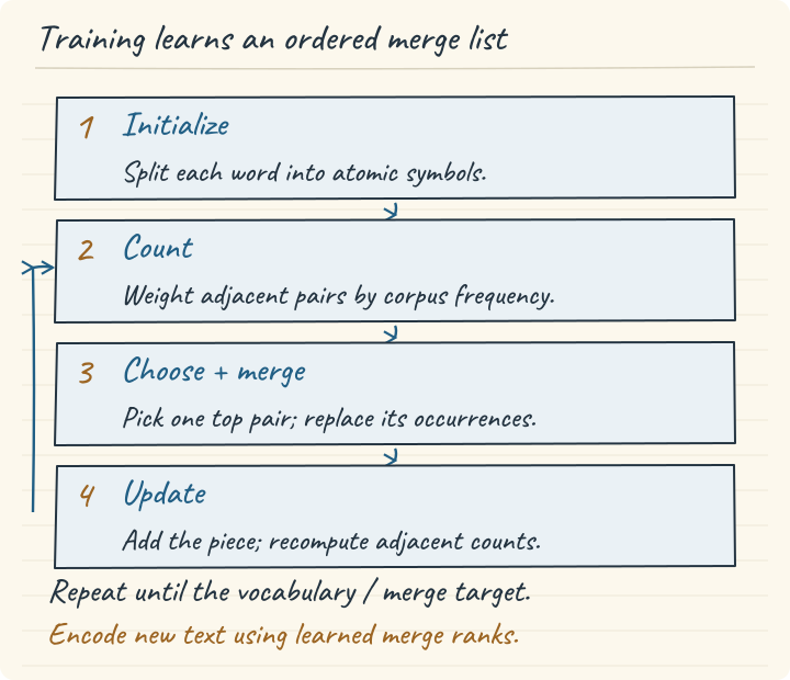
Recount after each merge: merging changes adjacency. New text uses the learned ranks rather than fresh corpus frequency counts.
Three initial pairs tie at frequency nine. Our deterministic rule chooses the lexicographically smallest pair among tied candidates, so e + s wins. Another tie rule can learn a different merge list. Determinism matters for reproducible examples and artifacts; a tied frequency does not mathematically force a unique vocabulary.
The first merge changes two words:
newest: n | e | w | e | s | t | </w>
                     └───┘
                 e + s → es
        n | e | w | es | t | </w>

widest: w | i | d | e | s | t | </w>
        w | i | d | es | t | </w>
The pair e + s no longer exists in those representations. Instead, w + es, d + es, and es + t appear. We must recompute counts using these new symbols, not continue using the original character table.
es + t has count nine and wins the next tie against t + </w>. After it is merged, est + </w> has count nine and becomes the third rule.
newest:
n | e | w | e | s | t | </w>   initial
n | e | w | es | t | </w>      rule 1
n | e | w | est | </w>         rule 2
n | e | w | est</w>            rule 3
est</w> is now a symbol containing the word-ending boundary. It is shared by newest and widest. The next strongest remaining shared pattern is in low and lower:
l | o | w | </w>        → lo | w | </w> → low | </w>
l | o | w | e | r | </w> → lo | w | e | r | </w> → low | e | r | </w>
The first eight learned rules, reproduced by the code below, are:
| Rank | Merge | Count when selected |
|---|---|---|
| 1 | e + s → es | 9 |
| 2 | es + t → est | 9 |
| 3 | est + </w> → est</w> | 9 |
| 4 | l + o → lo | 7 |
| 5 | lo + w → low | 7 |
| 6 | e + w → ew | 6 |
| 7 | ew + est</w> → ewest</w> | 6 |
| 8 | n + ewest</w> → newest</w> | 6 |
There are eleven base symbols, including </w>, and eight new merged symbols: a nineteen-symbol toy vocabulary. This count does not include extra padding or unknown tokens because this demonstration has not defined them.
A small implementation you can inspect
The following code is deliberately unoptimized. It makes every operation visible and avoids library internals. It uses Python’s standard library only. Each frequency remains attached to its current word representation.
from collections import Counter

word_frequencies = {"low": 5, "lower": 2, "newest": 6, "widest": 3}
initial_corpus = {
    tuple(word) + ("</w>",): frequency
    for word, frequency in word_frequencies.items()
}

def pair_counts(corpus):
    counts = Counter()
    for symbols, frequency in corpus.items():
        for pair in zip(symbols, symbols[1:]):
            counts[pair] += frequency
    return counts

def merge_symbols(symbols, pair):
    result = []
    index = 0
    while index < len(symbols):
        if (index + 1 < len(symbols)
                and (symbols[index], symbols[index + 1]) == pair):
            result.append("".join(pair))
            index += 2
        else:
            result.append(symbols[index])
            index += 1
    return tuple(result)

def train_bpe(corpus, merge_budget):
    corpus = dict(corpus)
    rules = []
    vocabulary = {symbol for word in corpus for symbol in word}
    history = []
    for _ in range(merge_budget):
        counts = pair_counts(corpus)
        if not counts:
            break
        pair = min(counts, key=lambda item: (-counts[item], item))
        rules.append(pair)
        vocabulary.add("".join(pair))
        updated = Counter()
        for symbols, frequency in corpus.items():
            updated[merge_symbols(symbols, pair)] += frequency
        corpus = dict(updated)
        history.append((pair, counts[pair], corpus.copy()))
    return rules, vocabulary, history

rules, vocabulary, history = train_bpe(initial_corpus, 8)
assert pair_counts({tuple("abab"): 9})[("a", "b")] == 18
assert pair_counts({tuple("aaaa"): 9})[("a", "a")] == 27
assert merge_symbols(tuple("aaaa"), ("a", "a")) == ("aa", "aa")
assert len(vocabulary) == 19

for rank, (pair, count, _) in enumerate(history, start=1):
    print(rank, pair, count)
Executed output:
1 ('e', 's') 9
2 ('es', 't') 9
3 ('est', '</w>') 9
4 ('l', 'o') 7
5 ('lo', 'w') 7
6 ('e', 'w') 6
7 ('ew', 'est</w>') 6
8 ('n', 'ewest</w>') 6
For intermediate corpus states, inspect history[step][2]. Replacing a pair preserves the original word frequency. The Counter used for the updated corpus also combines frequencies if multiple representations collapse to one key, rather than silently overwriting one.
Real trainers avoid recounting every pair in the entire corpus on every iteration. Efficient implementations maintain and update statistics. That engineering changes runtime substantially but does not change the central reasoning of this demonstration.
Applying learned merges to an unseen word
Training has produced an ordered rule list and a vocabulary. Encoding a new sentence does not restart training or ask which pair is most common in that sentence. It uses the already learned merge priorities.
Start with lowest, which never appeared in our training dictionary:
l | o | w | e | s | t | </w>
l | o | w | es | t | </w>      e+s
l | o | w | est | </w>         es+t
l | o | w | est</w>            est+</w>
lo | w | est</w>               l+o
low | est</w>                  lo+w
There is no rule merging low + est</w>. Both remaining pieces are in the learned vocabulary, so the new word is representable without a whole-word lowest entry.
For newer, the best applicable rule is e + w. The result after our eight-rule training run is:
n | ew | e | r | </w>This is more fragmented than newest, which eventually became one symbol. That difference follows from the training frequencies and limited merge budget. It is not proof that the tokenizer knows the comparative meaning of newer.
Here is a rank-based encoder using the already defined merge_symbols function:
def encode_word(word, rules, vocabulary):
    symbols = tuple(word) + ("</w>",)
    if any(symbol not in vocabulary for symbol in symbols):
        raise ValueError("Character absent from this toy alphabet")
    ranks = {pair: rank for rank, pair in enumerate(rules)}
    while True:
        candidates = [
            pair for pair in zip(symbols, symbols[1:])
            if pair in ranks
        ]
        if not candidates:
            return symbols
        pair = min(candidates, key=ranks.__getitem__)
        symbols = merge_symbols(symbols, pair)

print(encode_word("lowest", rules, vocabulary))
print(encode_word("newer", rules, vocabulary))
Executed output:
('low', 'est</w>')
('n', 'ew', 'e', 'r', '</w>')
The lowest rank is selected among applicable pairs. Frequency was relevant when learning those ranks; it is not recomputed here. The encoder remains limited to the known character alphabet. Try a word containing an unseen z and it deliberately raises an error. The next step fixes that coverage problem by changing the base units.
Unicode is not a tokenizer vocabulary
Python strings represent Unicode text. Unicode assigns abstract code points; UTF-8 is one encoding that represents Unicode scalar values using bytes. A byte contains eight bits and has possible values, numbered zero through 255.
Start with an ASCII character. c has code point U+0063, decimal 99. Its UTF-8 representation is a single byte of value 99. Here the code-point value and byte value happen to match. That coincidence stops outside ASCII.
For café, where é is the precomposed code point U+00E9:
| Character | Unicode code point | UTF-8 byte values, decimal | Bytes, hexadecimal |
|---|---|---|---|
c | U+0063 | 99 | 63 |
a | U+0061 | 97 | 61 |
f | U+0066 | 102 | 66 |
é | U+00E9 | 195, 169 | C3 A9 |
The string has four code points and five UTF-8 bytes. None of those values tells us an LLM tokenizer’s token IDs.
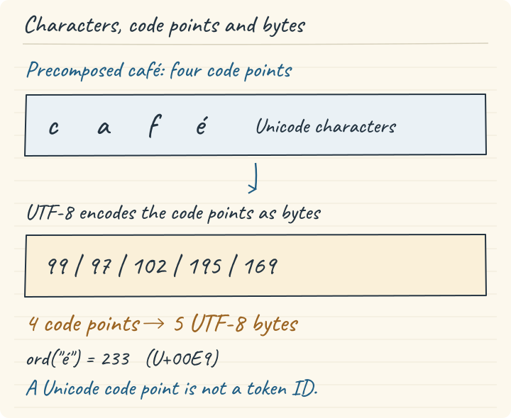
UTF-8 is an encoding of Unicode. The precomposed é occupies one code point and two bytes; a visible character can also use multiple code points.
text = "caf\u00e9"
print(len(text))
print([ord(character) for character in text])
print(list(text.encode("utf-8")))
print(ord("\u00e9"))
Executed output:
4
[99, 97, 102, 233]
[99, 97, 102, 195, 169]
233
ord("é") returns the Unicode code point 233. It does not return a tokenizer token ID. A particular tokenizer might encode that character as one token, several byte-containing tokens, or part of a longer piece including neighboring text.
The everyday word “character” also needs care. A visible é can be written as the precomposed code point U+00E9 or as e followed by combining acute accent U+0301. Those strings can look the same while having different code-point and byte sequences. Emoji can also combine multiple code points into one displayed grapheme.
import unicodedata

precomposed = "caf\u00e9"
decomposed = "cafe\u0301"
print(len(precomposed), len(decomposed))
print(precomposed == decomposed)
print(unicodedata.normalize("NFC", decomposed) == precomposed)
Executed output:
4 5
False
True
The tokenizer’s normalization policy decides whether these inputs become the same representation. NFC and NFKC are different policies with different preservation implications; do not add a normalizer simply to make a demonstration look cleaner. The Unicode standard defines the code-point and encoding distinctions, and Unicode normalization describes normalization forms.
Byte-level BPE changes the alphabet
Character BPE begins from characters. Byte-level BPE begins from byte representations. Its main merge idea is still to combine frequently adjacent units, but the starting coverage is different.
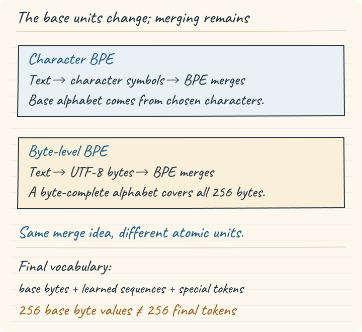
Full byte coverage provides a fallback for valid UTF-8 text. Normalization and implementation choices still determine exact round trips.
text → UTF-8 bytes → permitted byte spans → learned BPE merges → IDsIf all 256 byte values are representable and preprocessing preserves the input, every valid UTF-8 string can fall back to bytes. An unfamiliar writing system no longer requires a vocabulary entry for every character in that script before it can be represented. It can still be extremely inefficient if training learned few useful combinations for that script.
The base alphabet contains 256 possible byte values. The final vocabulary can contain many thousands of learned byte sequences plus special tokens. Saying “byte-level BPE has 256 tokens” confuses the fallback alphabet with the full learned inventory.
For café, the starting bytes are:
[99] [97] [102] [195] [169]Possible learned pieces might cover caf, é, or the entire word. These are possibilities, not output from a specified tokenizer. A learned token can also end midway through a multibyte character. Consequently, decoding an isolated token as UTF-8 may produce a replacement character, while decoding the concatenated byte sequence of all tokens reconstructs valid text.
Some implementations map byte values onto printable Unicode symbols internally. Those display symbols are labels for bytes; they do not turn the algorithm into ordinary character-level BPE. Inspect the implementation’s decoder rather than interpreting its token strings literally.
Byte fallback in a character-oriented tokenizer and a tokenizer trained entirely over byte representations are related coverage strategies, but they are not identical training designs. Likewise, being byte-complete does not imply an entire pipeline is lossless: normalization, trimming, special-token handling, or application-side transformations can still modify the input.
Boundaries and whitespace still matter
Byte coverage does not remove pre-tokenization. A regular expression may divide text into spans before BPE is applied. A byte-level tokenizer can attach a leading space to a word piece, separate digits into constrained groups, or prevent merges across punctuation. The exact tokenizer artifact is what defines the result.
This means token counts depend on context. cat in isolation may tokenize differently from cat after a space. A term list benchmark should therefore state whether terms are encoded alone, with a leading space, or in realistic sentences. We will use that distinction again when evaluating domain terminology.
For applications, the first useful tokenizer test is simple: encode realistic input, decode the whole sequence, and compare with the intended text. Then examine lengths and boundaries. A short sequence that silently drops an accent, a unit symbol, or a meaningful space has not met a preservation requirement merely because its token count is low.
tiktoken: a library, not a vocabulary
Byte-level BPE describes a way to construct and apply subword merges. A usable tokenizer also needs the actual vocabulary, merge ranks, text-boundary rules, and special-token handling. Those details determine which IDs a particular string receives. Two byte-level BPE tokenizers can agree on the algorithm while producing completely different IDs.
tiktoken is OpenAI’s tokenizer library; cl100k_base and o200k_base are named encodings loaded by that library. Selecting an encoding selects a particular set of rules and IDs. The library’s implementation operates on byte sequences and learned BPE ranks, with a regular-expression stage that restricts the regions within which merging occurs. OpenAI’s implementation makes that separation explicit.
This example deliberately names its encoding, so the result is reproducible without making a claim about whichever hosted model happens to be newest:
import tiktoken

encoding = tiktoken.get_encoding("cl100k_base")
text = "The cat chased the mouse."
ids = encoding.encode(text)
print(ids)
print([encoding.decode_single_token_bytes(i) for i in ids])
print(encoding.decode(ids))
Executed with tiktoken 0.14.0:
[791, 8415, 62920, 279, 8814, 13]
[b'The', b' cat', b' chased', b' the', b' mouse', b'.']
The cat chased the mouse.
The leading spaces belong to the bytes of these particular tokens. The ID 279 identifies b' the' in this encoding; it is neither a Unicode code point nor a universal ID for the English word “the.” Single-token bytes are useful for inspection because token boundaries can fall inside the UTF-8 encoding of a character. Decode the complete token sequence when reconstructing text. OpenAI’s tiktoken README documents the encoding API and the library’s BPE design.
WordPiece: frequency is not the only way to value a piece
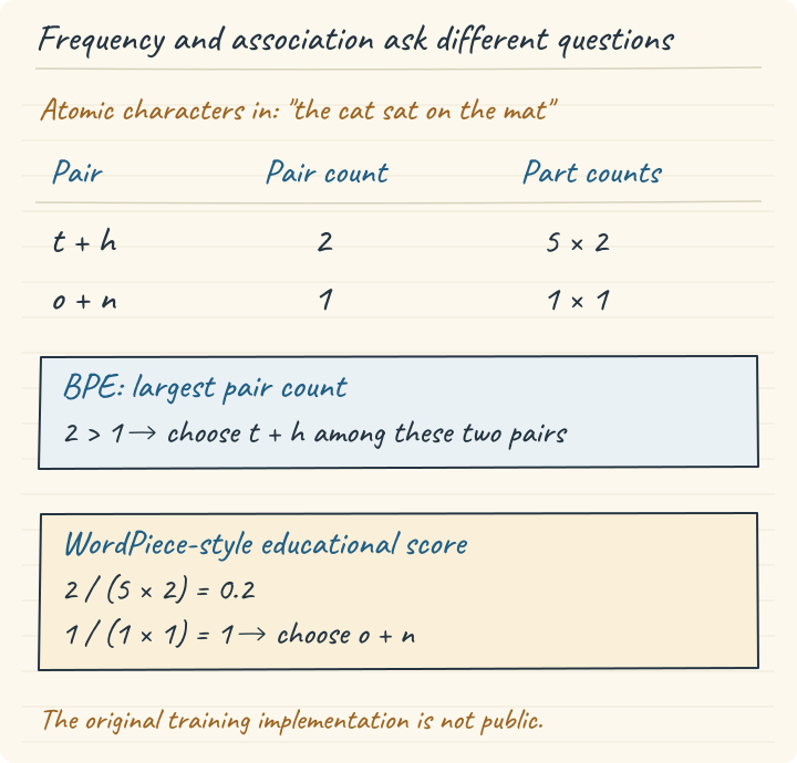
This two-pair comparison uses the educational normalized score. It is not a claim about a published canonical WordPiece trainer or a full-vocabulary merge decision.
BPE’s merge criterion rewards repeated adjacency. Consider a different question: is a pair especially associated with each other, relative to how often its members appear elsewhere? A common educational reconstruction of WordPiece training expresses this as
This formula is an explanatory model of WordPiece-style training. It should not be presented as an exact reproduction of Google’s original trainer: Google did not publicly release that training implementation, and the Hugging Face WordPiece course explicitly identifies its reconstruction as an approximation based on the literature.
For a numerical microscope, ignore spaces and use plain characters rather than continuation-marked pieces. In
the cat sat on the matthere are five t characters: one each in the, cat, sat, the second the, and mat. There are two h characters and two within-word th pairs. Consequently,
The characters o and n each occur once, and their pair occurs once:
Under this simplified criterion, on outranks th even though th is more frequent. The denominator discounts members that appear in many other combinations. This is association normalized by marginal counts, rather than raw pair frequency. It is not a semantic score: the arithmetic knows nothing about cats, mats, or grammatical meaning.
Here is the calculation without manually supplying the counts:
from collections import Counter

text = "the cat sat on the mat"
characters = Counter(text)
pairs = Counter(
    pair
    for word in text.split()
    for pair in zip(word, word[1:])
)

for a, b in [("t", "h"), ("o", "n")]:
    score = pairs[a, b] / (characters[a] * characters[b])
    print((a, b), characters[a], characters[b], pairs[a, b], score)
Verified output:
('t', 'h') 5 2 2 0.2
('o', 'n') 1 1 1 1.0
The simplified counting example isolates the criterion. A BERT-style WordPiece vocabulary distinguishes a word-initial piece from a continuation piece: play can begin a word, while ##ing marks a continuation. That marker is tokenizer notation, not two hash characters present in the original input.
Training and inference also need to be distinguished. BERT’s publicly available WordPiece tokenizer uses greedy longest-match-first segmentation: take the longest vocabulary piece matching the start of the remaining word; for later positions, search for continuation-marked entries. Continue until the word is covered. It consults the vocabulary, rather than replaying a BPE merge history. If a position cannot be covered, the original BERT implementation returns [UNK] for the whole pretokenized word, discarding partial pieces already found. It also has a word-length limit. These behaviors are directly inspectable in BERT’s tokenizer source.
For a deliberately tiny vocabulary containing [UNK], play, and ##ing, the Hugging Face WordPiece implementation produces:
playing → ['play', '##ing']
playz   → ['[UNK]']
These are executed results from that constructed vocabulary, not claims about the pretrained BERT vocabulary. The distinction matters when comparing WordPiece with byte-complete BPE: availability of every byte supplies the latter with a fallback that this tiny WordPiece vocabulary lacks.
SentencePiece: where the framework ends and the algorithm begins
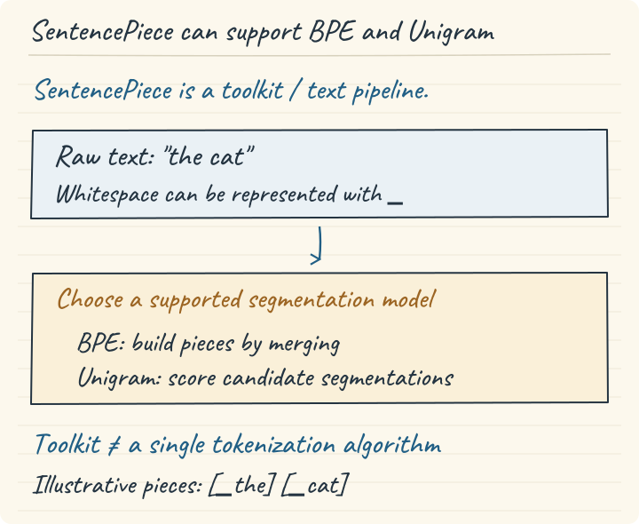
Whitespace handling and normalization are pipeline choices. The selected model determines how pieces are learned and segmented.
WordPiece notation assumes there is a meaningful word boundary before segmentation. But languages and datasets differ in how boundaries are written. A tokenizer pipeline should not require an English whitespace splitter to discover its subwords.
SentencePiece provides a framework for training from raw sentences, including normalization and whitespace handling. SentencePiece is the library; BPE and Unigram are alternative model types it supports. Seeing a .model file or the label “SentencePiece tokenizer” alone does not identify the underlying algorithm. Its repository also supports character and word model types. The SentencePiece paper explains the raw-sentence approach; the implementation’s README documents its model types.
SentencePiece makes spaces visible using the meta-symbol ▁ (U+2581). A schematic segmentation of the cat might be
▁the | ▁catThe exact pieces depend on the trained vocabulary. The marker records a boundary that would otherwise disappear when text was reduced to pieces. A dummy initial space is commonly added so a word at the start can receive the same treatment as a word following a space.
Normalization is part of this contract. SentencePiece commonly uses a normalization rule based on NFKC and has configurable whitespace processing. Its detokenizer reconstructs the normalized representation; preservation of arbitrary original spacing or compatibility-character distinctions depends on the chosen configuration. A successful encode/decode round trip must therefore be tested against the normalization policy, rather than assumed to preserve the original bytes. The official normalization and whitespace options expose these decisions.
Unigram: choose a good segmentation instead of following merges
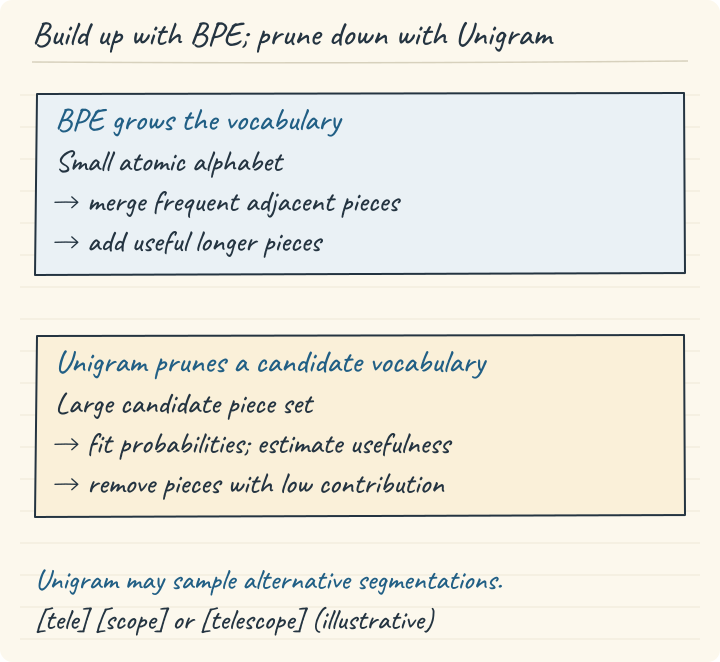
Both learn reusable pieces. Their training procedures differ; segmentation sampling can expose the model to alternate valid boundaries.
BPE grows a vocabulary by merging small pieces. Unigram begins with a larger set of candidate pieces and progressively prunes it while estimating which pieces help explain the corpus. Its learned object contains piece scores, rather than an ordered list of merge operations. The Unigram trainer exposes the probability-estimation and pruning stages.
For a segmentation , the Unigram model assigns a product of piece probabilities:
For one spelling, there may be several valid segmentations. The tokenization problem is to find the path with the highest score among those whose pieces concatenate to that spelling. In log space, multiplication becomes addition:
This explains both the name and the limits of the model. The segmentation score uses individual-piece probabilities. It is not the contextual probability assigned by the downstream Transformer to a sentence.
Consider an invented vocabulary containing telescope, tele, and scope. Suppose, solely for this arithmetic example,
P(telescope) = 0.006
P(tele)      = 0.080
P(scope)     = 0.050
The remaining vocabulary holds the remaining probability mass. Two candidate paths then receive scores
telescope      → 0.006
tele | scope   → 0.080 × 0.050 = 0.004
The first path wins between these candidates. Change the piece probabilities and the preferred path can change without changing the spelling. If the vocabulary includes additional pieces, there may be additional paths that must also be considered; the example is not an exhaustive segmentation of a real tokenizer.
An efficient implementation builds a lattice of matching pieces over positions in the string, then uses dynamic programming to find the best path. SentencePiece’s Unigram inference implementation implements this search and also supports alternative-path sampling. The vocabulary’s pieces need not coincide with linguistically meaningful morphemes: corpus fit drives their selection.
| Design question | BPE | Unigram |
|---|---|---|
| How does the vocabulary develop? | Add pieces through repeated pair merges | Start with candidates and prune while estimating piece scores |
| What is learned? | Vocabulary and merge ranking | Vocabulary and piece scores |
| How is ordinary inference performed? | Apply learned ranks to allowed regions | Find the highest-scoring complete segmentation |
Neither direction proves that an algorithm is universally better. Both are mechanisms for turning a corpus into a reusable segmentation rule. Evaluation still has to account for the data, normalization, boundary rules, vocabulary budget, and the model trained on the resulting IDs.
Subword regularization: expose the model to more than one spelling path
The ambiguity above can also become a training tool. Instead of always presenting a word through one segmentation, training can sample different valid paths from the same vocabulary. A vocabulary might support telescope, tele | scope, or finer alternatives. All can decode to the same normalized spelling while presenting different token sequences to the neural network.
Kudo’s subword regularization paper uses probabilistically sampled segmentations during neural machine translation training and reports improvements in its evaluated settings. This is a source-specific empirical result, not a promise that enabling sampling will improve every LLM. The idea resembles dropout in its use of training-time variation, but the sampled object here is the segmentation itself.
In our invented two-candidate example, their unnormalized scores were 0.006 and 0.004. Restricted to those two paths and without additional temperature adjustment, normalization gives probabilities 0.6 and 0.4. This arithmetic illustrates sampling; it is not an output from a trained SentencePiece model. Real sampling considers the paths available in that model and the configured distribution.
Production inference usually returns one deterministic segmentation unless sampling is intentionally enabled. Training data pipelines must make the policy explicit: tokenizer sampling changes token IDs and sequence lengths, so reproducibility requires recording its settings. A model trained only on one fixed tokenizer is not automatically ready for arbitrary segmentation changes at inference.
Vocabulary size buys shorter sequences at a price
Choosing BPE, WordPiece, or Unigram does not finish the design. Each still needs a vocabulary budget. A vocabulary with only atomic units can represent a sentence, but asks the model to process many positions. Adding reusable larger pieces can represent the same sentence with fewer positions. That trades sequence length against the number of distinct symbols the model must learn.
Consider an illustrative segmentation of acetylcholinesterase. One design might use six pieces, another three, another one. Those are three different sequence lengths for exactly the same spelling. The shortest representation saves positions in a fixed context window. It does not prove that the model has learned the enzyme’s function, and a tokenizer need not keep every specialized word whole.
The cost becomes concrete in the embedding matrix. With vocabulary size and embedding width , a dense input embedding contains parameters. At , the arithmetic is:
| Vocabulary | Input embedding parameters | BF16/FP16 storage for those weights |
|---|---|---|
| 16,000 | 65,536,000 | 125 MiB |
| 32,000 | 131,072,000 | 250 MiB |
| 50,000 | 204,800,000 | 390.625 MiB |
| 64,000 | 262,144,000 | 500 MiB |
| 100,000 | 409,600,000 | 781.25 MiB |
These are calculated examples, assuming two bytes per stored parameter; bytes. They exclude gradients, optimizer state, activation memory, and allocator overhead. A separate dense output projection adds approximately another weights; weight tying can share the input and output weights instead. The output layer must still produce vocabulary-sized scores when full logits are required.
There is also a sequence-side benefit. For a fixed text, fewer tokens can reduce attention work, KV-cache storage, and the number of autoregressive decoding steps. The net result depends on model size, attention implementation, batch size, hardware, and workload. A larger vocabulary can cost more per position while using fewer positions overall. A tokenizer compression benchmark measures one part of that balance, rather than determining a universal optimum. Research on code tokenizers explicitly studies this interaction between compression, vocabulary size, inference time, and memory. Dagan, Synnaeve, and Rozière
Vocabulary growth is useful when new slots capture recurring patterns. Spending slots on almost unique strings buys little held-out reuse. The design question becomes: which patterns deserve those slots for the text this system will actually process?
A vocabulary reflects the text that trained it
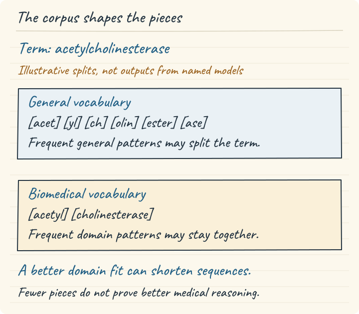
A domain tokenizer optimizes vocabulary coverage for its corpus. Efficient segmentation alone does not establish medical understanding.
A general English corpus contains many common verbs, names, places, and everyday expressions. A biomedical corpus changes the distribution: enzyme names, drug names, disease terms, gene identifiers, measurement units, and recurring scientific constructions appear much more often. Since subword training responds to corpus statistics, it can allocate larger pieces to these recurring domain patterns.
This is observable without training a language model. The following segmentations were reproduced from the released vocabularies of BERT-base-uncased and Microsoft’s abstract-only BiomedBERT, previously named PubMedBERT. Both are uncased WordPiece tokenizers. ## marks a continuation piece; it is tokenizer notation rather than literal text.
| Input | BERT-base-uncased | BiomedBERT, abstracts |
|---|---|---|
acetylcholinesterase | ace · ##ty · ##lch · ##olin · ##ester · ##ase | acetylcholinesterase |
amoxicillin | am · ##ox · ##ici · ##llin | amoxicillin |
echocardiography | echo · ##card · ##iography | echocardiography |
myocardial infarction | my · ##oca · ##rdial · in · ##far · ##ction | myocardial · infarction |
The first three inputs are single words. The last is a two-word term and remains two tokens in the biomedical tokenizer. “Domain vocabulary” therefore does not mean “every medical concept is one token.” The inputs here are lowercased and have no leading space; classification and separator tokens are excluded. The model vocabularies contain 30,522 and 28,895 entries respectively. This comparison illustrates different segmentation, while the unequal vocabulary sizes and different pretraining histories prevent treating it as a controlled causal experiment. BERT vocabulary, BiomedBERT vocabulary
The tokenizer has learned spelling patterns, not medical knowledge. A vocabulary entry for amoxicillin does not encode dosage, contraindications, or pharmacology. Those require the model’s learned representations and evidence from its training and context. Shorter segmentation changes the representation supplied to that model.
PubMedBERT’s authors studied domain vocabulary and domain pretraining together, including vocabulary ablations and input-length comparisons. That work supports investigating domain fit, but does not establish that any custom medical tokenizer automatically improves any medical task. A downstream result belongs to the complete training setup. Domain-Specific Language Model Pretraining for Biomedical Natural Language Processing
A clinical deployment can also receive appointment messages, administrative prose, mixed languages, and copied software logs. Optimizing only research abstracts may help one slice and harm another. This is why an evaluation needs both the home domain and the traffic that surrounds it.
Keep tokenizer training and evaluation separate
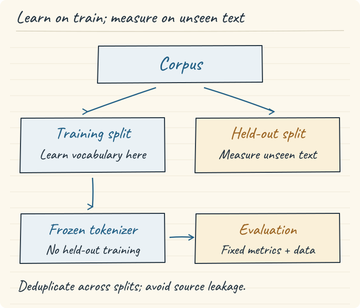
Training text measures fit to known data. Held-out text is needed to test whether that efficiency generalizes.
A tokenizer can memorize useful-looking pieces from its training text. Evaluating only on that text rewards this reuse without asking whether the vocabulary transfers to new examples. Reserve held-out text before counting pairs, fitting a Unigram model, selecting vocabulary size, or making normalization decisions.
The basic data boundary is:
Corpus
├── Training text → learn vocabulary and segmentation rules
├── Validation text → compare designs and select settings
└── Test text → estimate the selected design's final performance
The training and held-out sets may share ordinary words: learning frequent pieces that recur in new sentences is the purpose. What should be excluded is duplicated documents or closely copied passages masquerading as independent evidence. In biomedical data, split related records carefully: repeated versions of an abstract, papers from the same patient cohort, and templated reports can produce leakage.
Once vocabulary size is chosen by validation results, that validation set has participated in design selection. Use an untouched test set for the final claim. For an educational example, a clearly labeled train/validation comparison is enough to demonstrate the method; it is not enough to certify a production tokenizer.
There are two further boundaries. Do not truncate documents before counting tokens, because that can hide the very fragmentation being measured. Exclude automatically inserted special tokens when comparing segmentation efficiency, or report their overhead separately. A corpus with thousands of tiny records can otherwise appear inefficient largely because every record receives the same wrapper.
Measure splits, whole terms, and sequence length
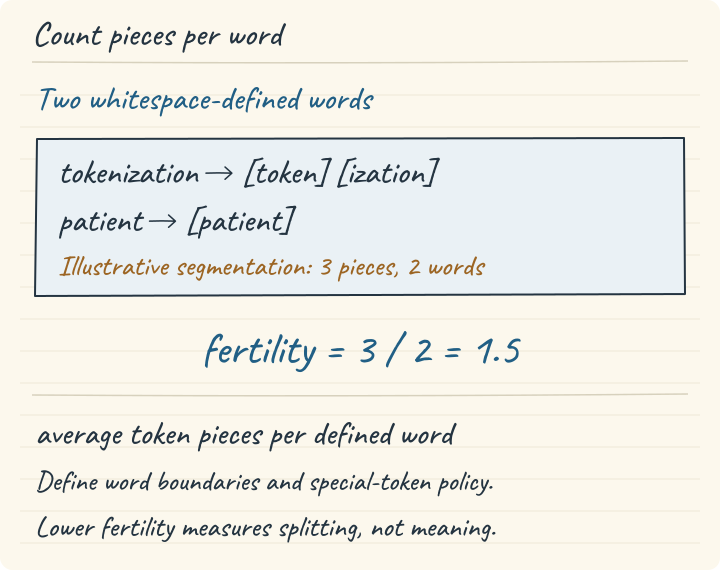
Use a documented word definition and a consistent policy for special tokens. Fertility is a segmentation-efficiency measure.
Fertility asks how many token pieces the tokenizer produces per reference word:
If patient becomes one token and tokenization becomes token · ization, those two words produce three pieces, giving fertility .
pieces = [["patient"], ["token", "ization"]]
fertility = sum(len(word_pieces) for word_pieces in pieces) / len(pieces)
print(fertility)
Executed output:
1.5That small example counts the pieces of already isolated words. In a corpus, define “word” before reporting a number. A whitespace split is an easy, reproducible English-oriented denominator, but treats patient. as one word and does not define words sensibly for every writing system. If the full tokenizer emits a separate punctuation token, that token appears in the numerator. Such a measurement is a text-token-to-whitespace-word ratio, not a pure measure of morphological fragmentation.
State whether you tokenize whole sentences or each reference word separately. Boundary-sensitive tokenizers can produce different pieces for patient and patient. Independently encoding words discards sentence context and whitespace behavior. Either protocol can answer a useful question, but their results should not be mixed.
Fertility should be aggregated deliberately. Suppose one document has ten words and twenty tokens, and another has ninety words and ninety tokens. Their individual fertilities are 2 and 1. The mean of document fertilities is 1.5, whereas corpus fertility is . The former weights the two documents equally; the latter weights reference words equally. Report which statistic you use.
Single-token rate asks a narrower question. For a curated list of target terms, count the terms represented by exactly one ordinary text token:
If heparin becomes [heparin], it is a hit; he · par · in is not. A list containing heparin, amoxicillin, and myocardial infarction may reasonably have a low rate for the last term because its space-separated words are kept apart. For that reason, report separate word and phrase coverage, or add mean pieces per term. Test bare and leading-space forms if both occur in deployment. A single [UNK] token is never a coverage success.
Finally, sequence efficiency asks how much text fits into the produced tokens. Define:
For an illustrative 1,000-character passage, 180 tokens gives 0.18 tokens per character; 240 gives 0.24. The first representation uses 25% fewer tokens: . For Unicode text, specify whether “character” means code point or grapheme cluster. Python’s len(text) counts code points. UTF-8 bytes per token is another reproducible metric:
Higher bytes per token indicates greater token efficiency. This is not a file-compression ratio: serializing token IDs, the vocabulary, and model weights has separate costs. Evaluation research uses normalized sequence length and bytes per token to compare tokenizers on fixed held-out text. Tokenizer compression metrics
None of these metrics measures semantic correctness. A tokenizer can preserve words elegantly while losing accents through normalization. Another can tokenize a long identifier into many pieces while preserving every byte. Check reconstruction and task behavior alongside token counts.
Train a byte-level domain BPE with an explicit contract
The following compact experiment uses Hugging Face tokenizers, tested here with version 0.23.1. It starts from all 256 byte values, uses ByteLevel pre-tokenization, preserves case, and uses the matching decoder. It intentionally has no lowercasing normalizer or special-token post-processor. This makes the encoding/decoding contract easy to inspect.
The vocab_size parameter is a target for the final vocabulary, including the initial alphabet and special tokens. It is not a count of merges. min_frequency prevents a candidate pair below that training frequency from receiving a merge. special_tokens reserves entries; it does not, by itself, insert those entries around each input. Small corpora can exhaust eligible merges before reaching the target. The trainer and ByteLevel APIs document these controls. BPE trainer, ByteLevel pre-tokenizer
from tokenizers import Tokenizer, decoders
from tokenizers.models import BPE
from tokenizers.pre_tokenizers import ByteLevel
from tokenizers.trainers import BpeTrainer

def train_bpe(documents, vocab_size=384):
    tokenizer = Tokenizer(BPE(unk_token="[UNK]"))
    tokenizer.pre_tokenizer = ByteLevel(add_prefix_space=False)
    tokenizer.decoder = decoders.ByteLevel()
    trainer = BpeTrainer(
        vocab_size=vocab_size,
        min_frequency=2,
        special_tokens=["[UNK]"],
        initial_alphabet=ByteLevel.alphabet(),
        show_progress=False,
    )
    tokenizer.train_from_iterator(documents, trainer=trainer)
    return tokenizer

def evaluate(tokenizer, documents):
    if not documents:
        raise ValueError("Provide at least one evaluation document.")
    counts = [
        len(tokenizer.encode(text, add_special_tokens=False).ids)
        for text in documents
    ]
    total_words = sum(len(text.split()) for text in documents)
    total_characters = sum(len(text) for text in documents)
    if not total_words or not total_characters:
        raise ValueError("Evaluation text must contain words and characters.")
    return {
        "tokens": sum(counts),
        "words": total_words,
        "characters": total_characters,
        "fertility": sum(counts) / total_words,
        "tokens_per_character": sum(counts) / total_characters,
        "average_tokens_per_document": sum(counts) / len(documents),
    }
The functions are reusable; their meaning depends on the corpus supplied. The following corpus is synthetic teaching text, not clinical records and not a biomedical benchmark. Its sentences are written to expose the mechanics of domain crossover. Repeating training sentences four times supplies pair-frequency support without introducing new information.
medical_train = [
    "The patient received amoxicillin for a bacterial infection.",
    "Echocardiography assessed myocardial function after myocardial infarction.",
    "Acetylcholinesterase inhibitors affect cholinergic signaling in neurons.",
    "The cardiologist reviewed echocardiography and electrocardiography results.",
    "Amoxicillin treatment reduced bacterial growth in the patient.",
    "Myocardial infarction can cause injury to cardiac tissue.",
    "The study measured acetylcholinesterase activity and enzyme inhibition.",
    "Clinical assessment included blood pressure and cardiac function.",
]
general_train = [
    "The gardener planted flowers beside the garden path.",
    "The children read a story about a village and a river.",
    "A traveler walked through the market during the morning.",
    "The school library collected books about history and music.",
    "The gardener watered the flowers and trimmed the trees.",
    "Children played beside the river after leaving school.",
    "The village market sold bread fruit and vegetables.",
    "A traveler visited the library to read a history book.",
]
medical_held_out = [
    "The patient had myocardial infarction.",
    "Amoxicillin was prescribed after clinical assessment.",
    "Echocardiography measured cardiac function.",
]
general_held_out = [
    "The children visited the garden.",
    "A traveler read a history book.",
    "The village market sold flowers.",
]
medical_bpe = train_bpe(medical_train * 4)
general_bpe = train_bpe(general_train * 4)
assert medical_bpe.get_vocab_size() == general_bpe.get_vocab_size() == 384

for name, tokenizer in [("medical", medical_bpe), ("general", general_bpe)]:
    for domain, documents in [
        ("medical", medical_held_out), ("general", general_held_out)
    ]:
        result = evaluate(tokenizer, documents)
        print(name, domain, result["tokens"], f'{result["fertility"]:.4f}')
Executed output:
medical medical 43 2.8667
medical general 67 4.1875
general medical 105 7.0000
general general 23 1.4375
To inspect a serialization round trip without leaving an example artifact behind:
from pathlib import Path
from tempfile import TemporaryDirectory

with TemporaryDirectory() as directory:
    path = Path(directory) / "tokenizer.json"
    medical_bpe.save(str(path))
    restored = Tokenizer.from_file(str(path))
    for text in ["Amoxicillin", " café", "Na+ 3.5 mg", "🙂"]:
        ids = restored.encode(text, add_special_tokens=False).ids
        assert restored.decode(ids) == text
    print("round trips passed")
Executed output:
round trips passedIn an actual project, save tokenizer.json at a stable versioned artifact location instead. Persist the corpus revision, split manifest, trainer settings, library version, and evaluation results with it. A vocabulary without its normalization, pre-tokenization, decoder, special-token behavior, and merge rules is an incomplete tokenizer.
The fair comparison is a two-by-two experiment
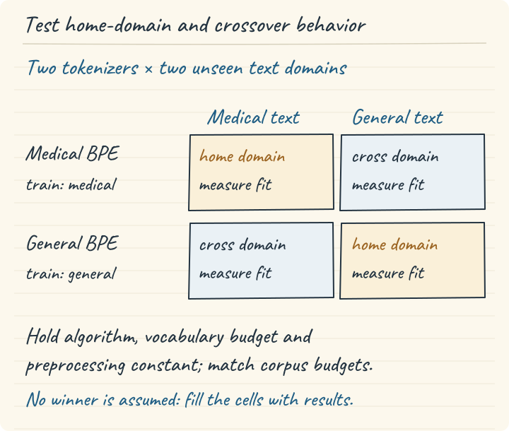
A fair comparison tests both domains under matched settings. Home-domain efficiency can come with a crossover cost.
Training two tokenizers with the same BPE algorithm, initial alphabet, pre-tokenizer, vocabulary size, frequency threshold, and special-token policy removes several confounders. Evaluate both on both held-out domains:
| Trained tokenizer | Medical held-out: tokens / fertility | General held-out: tokens / fertility |
|---|---|---|
| Medical BPE, 384 entries | 43 / 2.8667 | 67 / 4.1875 |
| General BPE, 384 entries | 105 / 7.0000 | 23 / 1.4375 |
These are measured results from the synthetic corpus above. The medical set has 15 whitespace words and 134 code points. The general set has 16 whitespace words and 95 code points. Compare tokenizers within a column, where the input is identical. Comparing 43 medical tokens with 23 general tokens would compare different text lengths and different distributions.
The medical tokenizer is more efficient on the medical examples; the general tokenizer is more efficient on the general examples. This is a home-domain crossover. Neither tokenizer wins universally. The artificial corpus intentionally makes that effect easy to see, so the size of the observed advantage must not be projected onto real medical traffic.
For a stronger study, equalize training data volume, deduplicate, use representative samples, and repeat across corpus draws. The small fixture uses equal numbers of sentences and repeats, but not equal character counts or equivalent diversity. An equal vocabulary budget alone does not make two corpora equally informative. Measure a mixture resembling deployment and also report each slice separately so that improvements on frequent text do not hide regressions on rare text.
Comparing two unrelated pretrained tokenizers can still answer an operational question: “Which checkpoint uses fewer tokens on this workload?” It does not isolate training domain. Their algorithms, normalization, vocabulary sizes, boundary rules, and special tokens may all differ. The two-by-two design makes the intended variable visible; model-quality claims require additional model training and task evaluation.
Sweep vocabulary size on actual held-out text
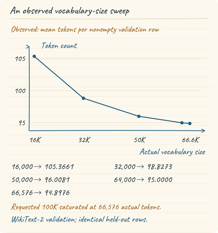
An observed WikiText-2 held-out sweep, not a medical-domain benchmark. The x-axis uses actual vocabulary sizes; a requested budget may exceed the number of learned pieces.
A good domain match does not tell us how many vocabulary entries to allocate. Train a family of tokenizers on the same training split while changing only the target vocabulary size. Evaluate each on identical held-out inputs.
The experiment below was executed on WikiText-2 raw, using Salesforce’s released dataset. Training used its training split; evaluation used its validation split. Empty or whitespace-only rows were removed. There were 23,767 nonempty training rows containing 10,892,990 code points, and 2,461 nonempty validation rows containing 1,142,150 code points. A row is the evaluation unit here: it is not necessarily a complete Wikipedia article. Thus “average tokens per row” should not be relabeled “average tokens per document.” WikiText dataset
This is a real general-text compression experiment. It is not a medical vocabulary recommendation, a language-model benchmark, or a reproduction of an uncited example curve. It uses tokenizers==0.23.1, the train_bpe function above, min_frequency=2, and no truncation or inserted special tokens.
| Requested vocabulary | Actual vocabulary | Mean tokens per held-out row | Change from previous target |
|---|---|---|---|
| 16K | 16,000 | 105.3661 | Baseline |
| 32K | 32,000 | 98.8273 | −6.21% |
| 50K | 50,000 | 96.0081 | −2.85% |
| 64K | 64,000 | 95.0000 | −1.05% |
| 100K | 66,576 | 94.8976 | −0.11% |
The last row is particularly useful. A request for 100,000 entries produced only 66,576. The available training text and frequency threshold exhausted eligible merges. Calling that a “100K tokenizer” would misdescribe the artifact. Any chart should use actual vocabulary on its horizontal axis, or explicitly label targets and realized sizes.
The measured counts across all validation rows were 259,306; 243,214; 236,276; 233,795; and 233,543 tokens respectively. The percentage change is computed from the unrounded totals or means:
where is the mean number of tokens for target . A negative change means fewer tokens. The early expansion captures relatively reusable pieces; later expansions buy smaller gains on this held-out text. This observed diminishing return is specific to the corpus and training configuration. A larger or different corpus could support the full 100K vocabulary and produce another curve.
Here is the complete data-loading and sweep code. It downloads two public Parquet files; it does not download model weights. Install requests and pyarrow in addition to tokenizers. The pinned dataset revision and expected file hashes make the exact input identifiable.
import hashlib
import io
import requests
import pyarrow.parquet as pq

revision = "b08601e04326c79dfdd32d625aee71d232d685c3"
expected = {
    "train": "e83889baabc497075506f91975be5fac0d45c5290b6b20582c8cd1e853d0c9f7",
    "validation": "204929b7ff9d6184953f867dedb860e40aa69c078fc1e54b3baaa8fb28511c4c",
}

def load_wikitext(split):
    url = (
        f"https://huggingface.co/datasets/Salesforce/wikitext/resolve/{revision}/"
        f"wikitext-2-raw-v1/{split}-00000-of-00001.parquet"
    )
    response = requests.get(url, timeout=90)
    response.raise_for_status()
    assert hashlib.sha256(response.content).hexdigest() == expected[split]
    rows = pq.read_table(io.BytesIO(response.content))["text"].to_pylist()
    return [text for text in rows if text.strip()]

wiki_train = load_wikitext("train")
wiki_validation = load_wikitext("validation")
sweep = []
previous = None
for target in [16_000, 32_000, 50_000, 64_000, 100_000]:
    tokenizer = train_bpe(wiki_train, vocab_size=target)
    total = sum(
        len(tokenizer.encode(text, add_special_tokens=False).ids)
        for text in wiki_validation
    )
    mean = total / len(wiki_validation)
    change = None if previous is None else 100 * (mean / previous - 1)
    sweep.append((target, tokenizer.get_vocab_size(), mean, total))
    print(target, tokenizer.get_vocab_size(), f"{mean:.4f}", total)
    previous = mean
Executed output:
16000 16000 105.3661 259306
32000 32000 98.8273 243214
50000 50000 96.0081 236276
64000 64000 95.0000 233795
100000 66576 94.8976 233543
Keep the evaluation text fixed across the sweep. If documents change length between runs, or if a larger tokenizer sees additional training data, the resulting curve no longer isolates vocabulary budget. Also check the actual artifact size after every run: a flat curve from saturated training is a different explanation from a full vocabulary adding pieces that do not help.
Select a practical knee without rounding away the decision
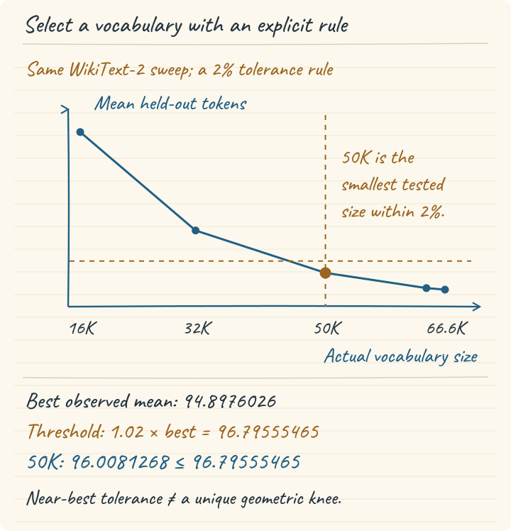
This 2% near-best rule selects 50K among the tested settings. It is a documented efficiency-cost decision, not proof of a unique geometric knee or an optimum for every task.
A knee is a useful region where additional vocabulary has relatively little efficiency benefit compared with its cost. It need not be a mathematically unique point. An explicit engineering rule is easier to review than choosing a visually appealing bend in a chart.
One possible rule is: choose the smallest tested vocabulary whose held-out mean token count is within 2% of the best observed count. The tolerance is a policy choice, not tokenizer theory.
For this sweep, the best mean is:
The allowable upper bound is:
The 32K tokenizer’s mean, 98.8273, is outside the band. The 50K tokenizer’s mean, 96.0081, is inside. The smallest tested qualifying vocabulary is therefore 50K. This is the result of a stated heuristic on this validation set. It is not evidence that 50K is optimal for biomedical text, multilingual text, or a particular deployed model.
best = min(row[2] for row in sweep)
threshold = best * 1.02
choice = min(
    (row for row in sweep if row[2] <= threshold),
    key=lambda row: row[1],  # Choose by realized vocabulary size.
)
print(f"threshold={threshold:.6f}, chosen_actual_vocab={choice[1]}")
Executed output:
threshold=96.795555, chosen_actual_vocab=50000Use full-precision values for selection and round for display afterward. To see why, consider a separate arithmetic example: a best value of 169.7 gives an exact 2% threshold of 173.094. A candidate value of 173.1 is slightly outside that band, even though both values display as 173.1 at one decimal place. Rounding the threshold first can change the selected vocabulary.
The tolerance also needs a workload interpretation. A 1% token-count difference can matter at very high volume, while a much larger embedding matrix can matter on a small device. Estimate real latency, memory, and task quality for the shortlisted settings. Repeat evaluation across documents or resampled corpora if small differences will drive an expensive decision.
A corpus must support the vocabulary it asks for
The sweep’s saturated final row makes a corpus-size issue visible: requesting more pieces does not create recurring evidence for them. Even when a trainer reaches a target, the tail of its vocabulary can be poorly supported.
For intuition only, suppose a corpus contains 6.3 million relevant counted units. Dividing that quantity by different vocabulary sizes gives:
| Vocabulary slots | Illustrative units per slot |
|---|---|
| 16K | 393.75 |
| 32K | 196.875 |
| 50K | 126 |
| 64K | 98.4375 |
| 100K | 63 |
This arithmetic is a budget metaphor. It is not a claim that each token is observed that many times, a confidence bound, a recommended sample size, or a theoretical vocabulary-selection rule. “Relevant counted units” must be defined before using such a ratio: words, bytes, characters, and tokens are different denominators, and token counts themselves depend on the tokenizer.
Actual frequencies are highly unequal. Frequent words and fragments occupy a large share of occurrences; many vocabulary entries sit in the tail. Moreover, BPE training frequencies describe the changing intermediate representation, while final emitted-token frequencies describe the trained tokenizer’s segmentation. A piece that was common early in training can later be absorbed into larger pieces.
Inspect final token frequencies, rare-piece coverage on held-out data, repeated boilerplate, and the realized vocabulary size. A corpus with many copies of one report can have substantial volume but little diversity. A smaller curated collection with broad terminology can offer different support. For the eventual model, rare token rows also require enough training occurrences to learn useful embeddings. A tokenizer’s training support and a language model’s embedding support are related questions, but they are not identical.
The tokenizer and pretrained model form one interface
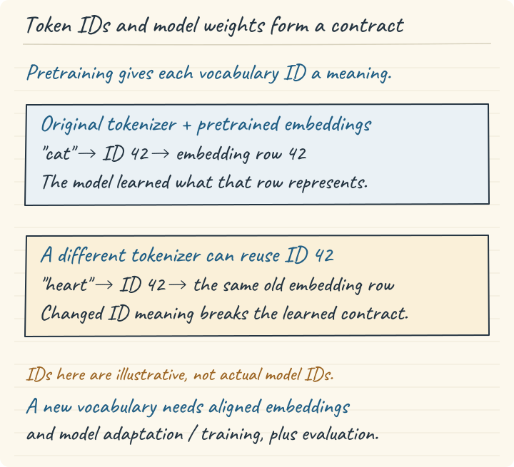
A custom tokenizer cannot be dropped into a pretrained model without aligning vocabulary-dependent weights and adapting and evaluating the model.
A newly trained domain tokenizer is usable immediately for inspecting text and measuring compression. It is not automatically compatible with an existing LLM.
Suppose tokenizer A maps token ID 1234 to patient. The pretrained model’s input embedding row 1234 was learned in contexts containing that token, and output logit 1234 means predicting it. If tokenizer B maps the same number to garden, the integer is in range but its meaning has changed.
Compatible pair
Tokenizer A: "patient" → ID 1234
Model A: row 1234 and output 1234 were trained for A's token.

Arbitrary replacement
Tokenizer B: "garden" → ID 1234
Model A: row 1234 still carries A's learned relationship.
The mismatch is not repaired by making both vocabularies the same size. Correct tensor shapes do not establish correct token semantics. Adding a larger embedding matrix only creates space for rows; it does not teach them. Special-token IDs, decoding rules, chat templates, and normalization can introduce additional incompatibilities.
There are valid routes, each with model-training work:
- Train a model from scratch with the chosen tokenizer so its input and output meanings are aligned from the start.
- Extend an existing vocabulary while preserving old IDs; initialize added rows deliberately, update input/output structures, and train the model to use those additions.
- Intentionally transfer to a modified vocabulary, initialize reusable pieces from compatible representations where possible, and continue pretraining before evaluating recovery and regressions.
The Transformers library offers embedding resizing as a structural operation. Research on tokenizer transfer and extension describes additional initialization and training strategies. Neither turns arbitrary tokenizer replacement into a safe drop-in operation. Embedding resizing, Tokenizer transfer and extension
For ordinary inference or fine-tuning of a released checkpoint, use its matching tokenizer and configuration. Keep custom-tokenizer evaluation separate until a model adaptation experiment is deliberately planned. The vocabulary defines the symbols; the pretrained model defines what it has learned to do with those symbols. Production correctness requires both to agree.
Representative tokenizer releases, with the counts kept honest
A Transformer architecture does not specify its tokenizer. The following table names particular published releases or documented encodings, rather than claiming one tokenizer for every generation of a family. “Vocabulary size” can mean mergeable entries, all tokenizer IDs, or model embedding/output rows; those quantities need not agree. Artifact counts below were inspected on 7 October 2026.
| Named release or encoding | Family / implementation | Vocabulary accounting | Source and caution |
|---|---|---|---|
OpenAI | tiktoken byte-level BPE | 100,256; 199,998 mergeable entries, respectively | Encoding definitions . Special IDs and gaps make |
| Meta Llama 3, original 8B/70B release | tiktoken-based byte-level BPE | 128,000 base entries + 256 reserved/special IDs = 128,256 | Meta implementation . Do not transfer this to Llama 2, which uses SentencePiece. |
| Qwen2.5-7B | Hugging Face byte-level BPE | 151,643 core entries; 151,665 total tokenizer IDs; 152,064 model rows | Tokenizer and config . Other sizes/releases can allocate different model rows. |
| DeepSeek-V3, original published checkpoint | Hugging Face BPE with ByteLevel preprocessing/decoding | 128,000 core entries; 128,815 distinct tokenizer IDs; 129,280 model rows | Tokenizer and config . Added-token records overlap some core IDs, so do not simply add record counts. |
| Gemma 2 | SentencePiece-compatible BPE with byte fallback | 256,000 model vocabulary rows | Google config and Hugging Face implementation . The gated tokenizer artifact was not downloaded in this audit. |
| Mistral-7B-v0.1 | SentencePiece-compatible BPE with byte fallback | 32,000 core/model entries | Original tokenizer artifact . Newer Mistral releases can use tiktoken-based Tekken; Mistral’s documentation distinguishes these versions. |
| BERT-base-uncased | WordPiece | 30,522 entries/model rows | Named checkpoint config . Cased and multilingual BERT have different vocabularies. |
| T5-base | SentencePiece Unigram | 32,000 SentencePiece entries + 100 sentinel IDs = 32,100 tokenizer IDs; 32,128 model rows | Tokenizer artifact , model config , and T5 tokenizer documentation . The additional model rows are not 28 extra learned text pieces. |
For an undocumented proprietary tokenizer, the correct entry is “proprietary / not publicly specified.” A familiar model name, a decoder-only architecture, or an approximate vocabulary count is insufficient evidence to fill in its algorithm. These distinctions become practical when comparing efficiency: compare the complete configured tokenizer on held-out text, and verify that its IDs remain compatible with the model consuming them.
A tokenizer is part of the model contract
It is useful to separate three questions before making a tokenizer decision:
- Can the tokenizer preserve and represent the intended input?
- Does it encode the workload efficiently under an acceptable vocabulary budget?
- Was the model trained, or intentionally adapted, to consume exactly those IDs?
A tokenizer can pass the first two checks and fail the third. That is why a domain tokenizer trained in a few seconds is not automatically an upgrade to an existing LLM. Compression is a property of a tokenizer and text distribution; useful prediction is a property of a trained model and its complete input contract.
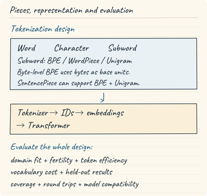
Tokenizer quality is a property of the full pipeline and its intended use, not a single compression score.
The family relationships are:
TEXT
 ├─ word units
 ├─ character units
 └─ subword units
     ├─ BPE: grow pieces through ordered merges
     │   └─ byte-level BPE: use byte representations as base units
     ├─ WordPiece: learned vocabulary, greedy longest-match encoding
     └─ Unigram: probabilistic pieces and segmentation search

SentencePiece: a framework supporting several models, including BPE and Unigram
tiktoken: an implementation/library exposing named BPE encodings

text → tokenizer pipeline → IDs → learned embeddings → Transformer
Algorithm, implementation, encoding, and model checkpoint are different levels of description. “SentencePiece” alone does not say whether the trained model uses BPE or Unigram. “tiktoken” alone does not specify which encoding is loaded. “Decoder-only Transformer” does not determine any tokenizer algorithm.
For a new model, choose and version the full tokenizer before pretraining, and evaluate on text reflecting the intended workload. For an existing model, start from its released tokenizer and chat template. For research on replacement, make vocabulary adaptation and model retraining part of the experiment rather than an invisible preprocessing change.
What to retain for an engineering interview
Why do corpus frequencies multiply pair counts? A frequency dictionary compresses repeated observations. If a pair appears twice in a spelling that occurs nine times, the corpus has eighteen such pair occurrences. Ignoring the multiplier trains on a different distribution.
What changes between BPE training and encoding? Training counts adjacent pairs and learns merge priorities. Encoding applies those learned priorities to new text. It does not learn a fresh vocabulary from each prompt.
Why do bytes help with OOV? A complete 256-value fallback alphabet can represent UTF-8 text without requiring every Unicode character as an initial learned entry. Coverage still says nothing about how efficiently an underrepresented language is segmented.
Why can WordPiece prefer a rarer pair? The educational association score divides pair frequency by the product of its component frequencies. Relative association and raw occurrence count can rank candidates differently. Exact trainer details must still be identified rather than assumed from that teaching formula.
Why is fertility not a quality score? It reports fragmentation relative to a specified word-count convention. It does not measure whether a model knows the domain, whether normalization preserved information, or whether the vocabulary cost is justified.
How do you choose a vocabulary size? Train controlled candidates, record realized sizes, evaluate on a held-out selection split, measure sequence lengths and practical costs, then select under an explicit budget or tolerance. Keep a final test split untouched. A knee heuristic is a decision rule, not a universal optimum.
Why can you not swap tokenizers freely? The same ID can refer to a different string in another vocabulary. The input embedding and output prediction rows were learned under the original assignment. Changing segmentation and assignments changes what the model reads and emits.
These answers connect back to one mechanism: a tokenizer allocates a finite set of discrete units to a distribution of text. Good engineering requires preserving the text, measuring the allocation on unseen data, and maintaining the model’s agreement about what every unit means.