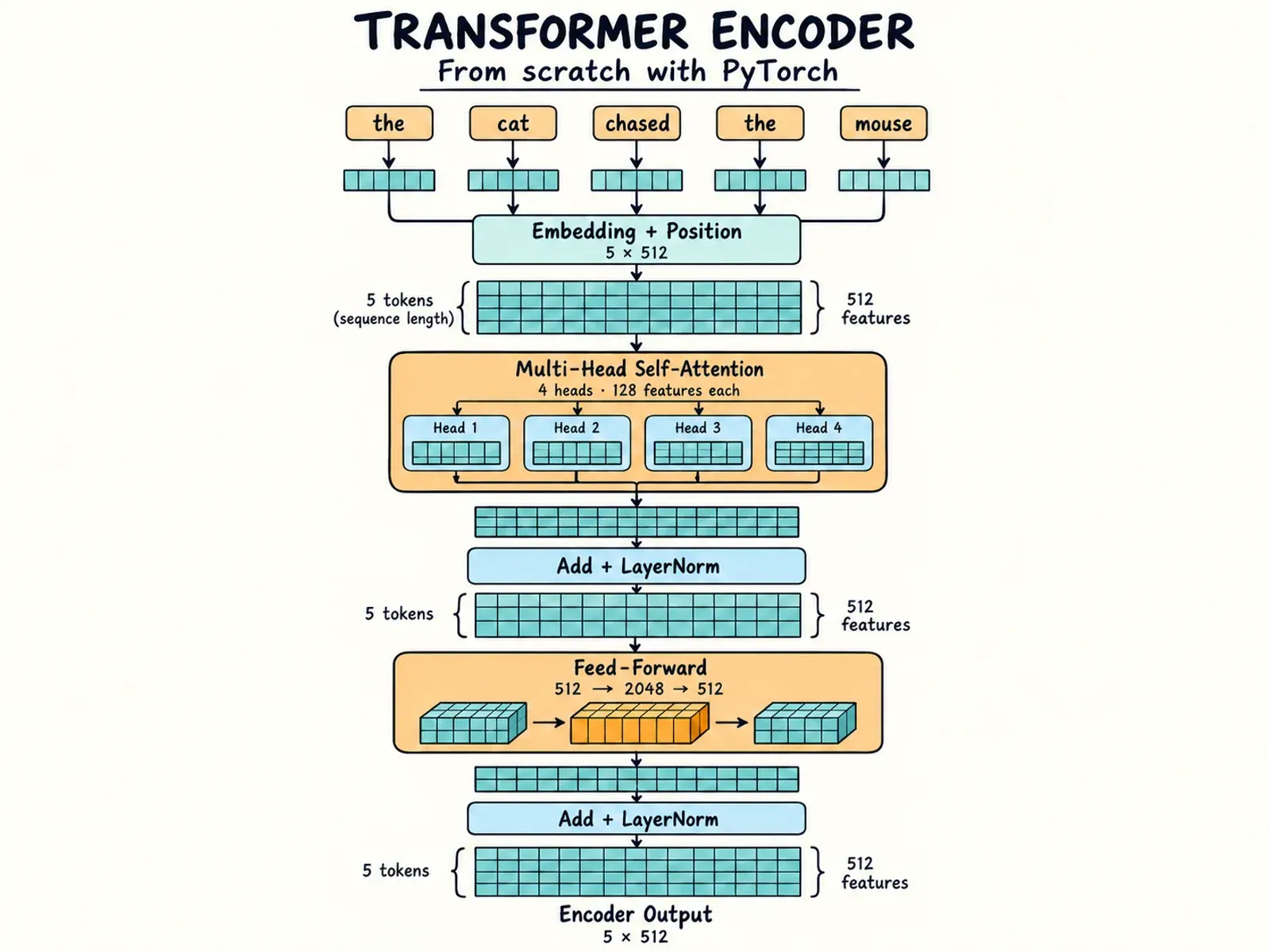
What this encoder does
A Transformer encoder uses self-attention to mix information between tokens and a feed-forward network to transform each token’s features. We will implement its forward pass with basic PyTorch tensor operations, following “The cat chased the mouse” from token IDs to a 5 × 512 output.
The illustration above is a simplified overview of the stages. Each Add also receives the input to its own sublayer through a residual path; the equations and code below show those two additions explicitly.
Run the notebook
Download the original notebook, including its saved outputs.
Install the two dependencies in your Python environment, then open the notebook and run its cells from top to bottom:
python -m pip install torch richThe numbered walkthrough’s Python blocks follow the same execution order. Later blocks reuse definitions from earlier ones; the PyTorch glossary also contains illustrative fragments, which are not standalone programs. The expandable output blocks reproduce the supplied notebook’s saved run, with terminal color escapes removed; they are not live computations in your browser. That saved run reports PyTorch 2.14.0+cpu. Values can vary across versions, devices, and seeds.
The initial walkthrough uses seed 7; the factory example later resets the seed to 42 and constructs a fresh model. Their numeric outputs are therefore different even though their shapes and operations agree.
Encoder overview
This notebook builds a complete Transformer Encoder from scratch using PyTorch, with the goal of understanding what actually happens inside the architecture instead of treating it as a black box.
We will use the simple sentence:
“The cat chased the mouse”
and follow it through every major encoder stage:
The notebook focuses on the forward pass and makes the intermediate tensors, dimensions, and calculations visible using Rich printing.
Configuration used in this notebook
For our example:
Therefore:
and the Feed-Forward Network uses:
So the main configuration is:
- Sequence length:
- Model dimension:
- Number of attention heads:
- Dimension per head:
- Feed-Forward hidden dimension:
Why build the encoder from scratch?
PyTorch already provides high-level components such as:
nn.MultiheadAttention
nn.LayerNorm
nn.TransformerEncoderLayer
nn.TransformerEncoder
But if we use those directly, many important Transformer operations become hidden.
In this notebook, we deliberately implement the core logic ourselves so we can clearly see:
- how token embeddings are created
- how positional information is added
- how Query, Key, and Value are produced
- how attention scores are calculated
- why we divide by
- how Softmax produces attention weights
- how multiple heads are split and concatenated
- how residual connections work
- how LayerNorm works
- how the Feed-Forward Network transforms features
- how the final contextual token representations are produced
So the purpose is not only to run an encoder, but to understand:
what each tensor means, why each operation exists, and how the dimensions move through the architecture.
What does a Transformer Encoder do?
A Transformer Encoder converts ordinary token representations into context-aware token representations.
At the beginning, a token mainly represents:
After adding positional information, it also knows:
After Self-Attention, it can incorporate information from other tokens:
After the Feed-Forward Network, its contextual features are transformed further.
So the final representation answers something closer to:
Example intuition
Consider the sentence:
“The cat chased the mouse”
The token:
“chased”
does not need to be understood in isolation.
Through Self-Attention, its representation can be influenced by:
“cat”
and:
“mouse”
because those tokens are relevant to the meaning of the action.
Likewise, the word:
“the”
appears twice.
Before positional information is added, both occurrences may begin with the same token embedding.
But after positional encoding and contextual processing, their representations can become different because they appear at different positions and interact with different surrounding tokens.
This is the central idea of the encoder:
Encoder flow
The full encoder pipeline we will build is:
Raw Sentence
     ↓
Tokenization
     ↓
Token IDs
     ↓
Token Embeddings
     ↓
+ Positional Encoding
     ↓
Encoder Input X
     ↓
Create Q, K, V
     ↓
Split into Multiple Heads
     ↓
Scaled Dot-Product Attention
     ↓
Softmax Attention Weights
     ↓
Attention × Value
     ↓
Concatenate Heads
     ↓
Output Projection
     ↓
Residual Connection
     ↓
LayerNorm
     ↓
Feed-Forward Network
     ↓
Second Residual Connection
     ↓
Second LayerNorm
     ↓
Final Encoder Output
The final output has shape:
The shape is similar to the main input representation, but the information stored inside each vector is much richer.
Important encoder property
Unlike an autoregressive decoder, a standard encoder normally does not use a causal mask.
That means each token can attend to tokens on both the left and the right.
For example:
“chased”
can attend to both:
“cat”
and:
“mouse”
at the same time.
So encoder self-attention is generally:
Padding masks may still be used when sequences in a batch have different lengths.
Common encoder use cases
Transformer encoders are useful whenever we want strong contextual representations of text.
Typical applications include:
-
Text classification sentiment analysis, spam detection, intent detection, topic classification
-
Token classification Named Entity Recognition, POS tagging, sequence labeling
-
Semantic search and retrieval sentence embeddings, document embeddings, similarity search, RAG retrieval
-
Extractive question answering
-
Encoder-decoder architectures where the encoder produces a contextual memory that the decoder reads through cross-attention
What we will learn
By the end of this notebook, we will understand not just:
what a Transformer Encoder contains
but also:
why each component exists, how its mathematics works, and how its tensor dimensions fit together.
The goal is to move from:
to:
Environment setup
# If needed in a fresh environment, install dependencies with:
# !pip install torch rich

import math
import random
import torch
import torch.nn as nn
import torch.nn.functional as F

from rich.console import Console
from rich.panel import Panel
from rich.table import Table
from rich import box

console = Console(width=140)

torch.manual_seed(7)
random.seed(7)

device = torch.device("cuda" if torch.cuda.is_available() else "cpu")

console.print(Panel.fit(
    f"[bold green]Environment ready[/bold green]\n"
    f"PyTorch: {torch.__version__}\n"
    f"Device: {device}",
    title="Setup"
))
Show saved notebook output
╭─────── Setup ───────╮
│ Environment ready   │
│ PyTorch: 2.14.0+cpu │
│ Device: cpu         │
╰─────────────────────╯
1. Configuration and the simple sentence
We lowercase the sentence so both occurrences of “the” map to the same token ID. This makes it easy to see how position + attention later make their representations different.
SENTENCE = "The cat chased the mouse"
D_MODEL = 512
NUM_HEADS = 4
D_HEAD = D_MODEL // NUM_HEADS
D_FF = 2048
NUM_LAYERS = 1

assert D_MODEL % NUM_HEADS == 0

def simple_tokenize(sentence: str):
    """Very small educational tokenizer: lowercase + whitespace split."""
    return sentence.lower().strip().split()

def build_vocab(tokens):
    vocab = {"<pad>": 0, "<unk>": 1}
    for tok in tokens:
        if tok not in vocab:
            vocab[tok] = len(vocab)
    return vocab

def tokens_to_ids(tokens, vocab):
    return torch.tensor([vocab.get(tok, vocab["<unk>"]) for tok in tokens], dtype=torch.long, device=device)

tokens = simple_tokenize(SENTENCE)
vocab = build_vocab(tokens)
token_ids = tokens_to_ids(tokens, vocab)
N = len(tokens)

config_table = Table(title="Encoder Configuration", box=box.ROUNDED)
config_table.add_column("Item", style="bold cyan")
config_table.add_column("Value", style="white")
for k, v in [
    ("Sentence", SENTENCE),
    ("Tokens", str(tokens)),
    ("Token IDs", str(token_ids.tolist())),
    ("n", str(N)),
    ("d_model", str(D_MODEL)),
    ("heads", str(NUM_HEADS)),
    ("d_k = d_v", str(D_HEAD)),
    ("d_ff", str(D_FF)),
]:
    config_table.add_row(k, v)
console.print(config_table)

console.print("\n[bold]Vocabulary[/bold]")
for token, idx in vocab.items():
    console.print(f"  {token!r:>8} -> {idx}")
Show saved notebook output
                 Encoder Configuration
╭───────────┬──────────────────────────────────────────╮
│ Item      │ Value                                    │
├───────────┼──────────────────────────────────────────┤
│ Sentence  │ The cat chased the mouse                 │
│ Tokens    │ ['the', 'cat', 'chased', 'the', 'mouse'] │
│ Token IDs │ [2, 3, 4, 2, 5]                          │
│ n         │ 5                                        │
│ d_model   │ 512                                      │
│ heads     │ 4                                        │
│ d_k = d_v │ 128                                      │
│ d_ff      │ 2048                                     │
╰───────────┴──────────────────────────────────────────╯


Vocabulary

   '<pad>' -> 0

   '<unk>' -> 1

     'the' -> 2

     'cat' -> 3

  'chased' -> 4

   'mouse' -> 5
Rich tensor-printing helpers
A 5 × 512 matrix contains 2,560 numbers, so dumping every number makes the notebook unreadable. The helper below prints every important step, its shape, and a useful slice of values.
Set SHOW_FULL_512 = True if you really want all 512 columns printed.
SHOW_FULL_512 = False
PREVIEW_COLS = 8

def rich_tensor(name, tensor, row_labels=None, max_rows=8, max_cols=PREVIEW_COLS, precision=4):
    t = tensor.detach().cpu()
    if t.ndim == 1:
        t = t.unsqueeze(0)
    if t.ndim != 2:
        console.print(f"[bold yellow]{name}[/bold yellow] shape={tuple(tensor.shape)}")
        console.print(t)
        return

    rows, cols = t.shape
    show_rows = rows if SHOW_FULL_512 else min(rows, max_rows)
    show_cols = cols if SHOW_FULL_512 else min(cols, max_cols)

    table = Table(title=f"{name}   shape={tuple(tensor.shape)}", box=box.SIMPLE_HEAVY)
    table.add_column("row", style="bold cyan")
    for j in range(show_cols):
        table.add_column(str(j), justify="right")
    if show_cols < cols:
        table.add_column("…", justify="center")

    for i in range(show_rows):
        label = row_labels[i] if row_labels and i < len(row_labels) else str(i)
        vals = [f"{float(t[i, j]):.{precision}f}" for j in range(show_cols)]
        if show_cols < cols:
            vals.append("…")
        table.add_row(str(label), *vals)

    if show_rows < rows:
        table.add_row("…", *(["…"] * (show_cols + (1 if show_cols < cols else 0))))
    console.print(table)


def rich_attention_matrix(name, matrix, tokens):
    """Print a complete n×n attention-score/weight matrix for our short sentence."""
    m = matrix.detach().cpu()
    table = Table(title=f"{name}   shape={tuple(matrix.shape)}", box=box.ROUNDED)
    table.add_column("Q \\ K", style="bold cyan")
    for tok in tokens:
        table.add_column(tok, justify="right")
    for i, tok in enumerate(tokens):
        table.add_row(tok, *[f"{float(m[i, j]):.4f}" for j in range(len(tokens))])
    console.print(table)


def print_shape_equation(label, equation):
    console.print(f"[bold magenta]{label}[/bold magenta]  {equation}")
2. Input token embeddings
An embedding table stores one trainable vector for each vocabulary item.
For a token ID :
where:
- = vocabulary size
- each token is represented by a vector of 512 numbers
For our example:
“The cat chased the mouse”
we have:
tokens.
Therefore, the embedding matrix has shape:
So:
This means:
- rows = one row for each token
- columns = 512 embedding features for each token
Conceptually:
where each row has:
learned values.
Because our simple tokenizer lowercases the sentence, repeated occurrences of the same token initially receive the same token embedding.
For example:
At this stage, the model knows:
what the token is
but it does not yet know:
where the token appears in the sentence
Later, positional encoding adds this position information.
class ManualEmbedding(nn.Module):
    def __init__(self, vocab_size, d_model):
        super().__init__()
        self.weight = nn.Parameter(torch.randn(vocab_size, d_model) * 0.02)

    def forward(self, token_ids):
        # Direct row lookup from the trainable embedding matrix.
        return self.weight[token_ids]

embedding_layer = ManualEmbedding(len(vocab), D_MODEL).to(device)
token_embeddings = embedding_layer(token_ids)

console.print(Panel.fit("[bold]STEP 1 — TOKEN EMBEDDINGS[/bold]", border_style="green"))
print_shape_equation("Shape", f"token_ids {tuple(token_ids.shape)} -> embeddings {tuple(token_embeddings.shape)} = [n, d_model]")
rich_tensor("Token embeddings E[token_id]", token_embeddings, row_labels=tokens)

same = torch.allclose(token_embeddings[0], token_embeddings[3])
console.print(f"\nBoth 'the' token embeddings identical before position information? [bold]{same}[/bold]")
Show saved notebook output
╭───────────────────────────╮
│ STEP 1 — TOKEN EMBEDDINGS │
╰───────────────────────────╯

Shape  token_ids (5,) -> embeddings (5, 512) =

                             Token embeddings E   shape=(5, 512)

  row            0         1         2         3         4         5         6         7   …
 ━━━━━━━━━━━━━━━━━━━━━━━━━━━━━━━━━━━━━━━━━━━━━━━━━━━━━━━━━━━━━━━━━━━━━━━━━━━━━━━━━━━━━━━━━━━━
  the       0.0170    0.0022    0.0268    0.0356    0.0132   -0.0050    0.0252    0.0307   …
  cat      -0.0075    0.0155    0.0094   -0.0118   -0.0361    0.0209    0.0220    0.0101   …
  chased   -0.0248    0.0157   -0.0056    0.0010    0.0107    0.0081   -0.0321   -0.0069   …
  the       0.0170    0.0022    0.0268    0.0356    0.0132   -0.0050    0.0252    0.0307   …
  mouse    -0.0031   -0.0182   -0.0324   -0.0578   -0.0040    0.0133   -0.0276   -0.0051   …


Both 'the' token embeddings identical before position information? True
3. Positional encoding
Self-attention by itself does not know the order of tokens.
For example, without positional information, the model does not inherently know whether a token appeared:
- first
- second
- third
- fifth
So we add a positional encoding vector to every token embedding.
For even dimensions:
For odd dimensions:
where:
- = position of the token in the sentence
- = embedding dimension index
For our sentence:
“The cat chased the mouse”
the token positions are:
Token | Position |
|---|---|
The | 0 |
cat | 1 |
chased | 2 |
the | 3 |
mouse | 4 |
Since:
and:
the positional encoding matrix has shape:
Each row represents the positional information for one token.
So conceptually:
where every:
The positional encoding has the same shape as the token embeddings, because in the next step we will add them element-wise:
def sinusoidal_positional_encoding(seq_len, d_model, device):
    pe = torch.zeros(seq_len, d_model, device=device)
    position = torch.arange(seq_len, dtype=torch.float32, device=device).unsqueeze(1)
    div_term = torch.exp(
        torch.arange(0, d_model, 2, dtype=torch.float32, device=device)
        * (-math.log(10000.0) / d_model)
    )
    pe[:, 0::2] = torch.sin(position * div_term)
    pe[:, 1::2] = torch.cos(position * div_term)
    return pe

positional_encoding = sinusoidal_positional_encoding(N, D_MODEL, device)

console.print(Panel.fit("[bold]STEP 2 — POSITIONAL ENCODING[/bold]", border_style="green"))
rich_tensor("Positional encoding PE", positional_encoding, row_labels=[f"pos {i}" for i in range(N)])
Show saved notebook output
╭──────────────────────────────╮
│ STEP 2 — POSITIONAL ENCODING │
╰──────────────────────────────╯

                           Positional encoding PE   shape=(5, 512)

  row           0         1         2         3         4         5         6         7   …
 ━━━━━━━━━━━━━━━━━━━━━━━━━━━━━━━━━━━━━━━━━━━━━━━━━━━━━━━━━━━━━━━━━━━━━━━━━━━━━━━━━━━━━━━━━━━
  pos 0    0.0000    1.0000    0.0000    1.0000    0.0000    1.0000    0.0000    1.0000   …
  pos 1    0.8415    0.5403    0.8219    0.5697    0.8020    0.5974    0.7819    0.6234   …
  pos 2    0.9093   -0.4161    0.9364   -0.3509    0.9581   -0.2863    0.9749   -0.2227   …
  pos 3    0.1411   -0.9900    0.2451   -0.9695    0.3428   -0.9394    0.4336   -0.9011   …
  pos 4   -0.7568   -0.6536   -0.6572   -0.7537   -0.5486   -0.8361   -0.4342   -0.9008   …
4. Add token embeddings + positional encoding
Before the input enters the encoder’s self-attention block, we combine two pieces of information:
- What the token is → Token Embedding
- Where the token appears → Positional Encoding
The final encoder input is:
For our sentence:
“The cat chased the mouse”
we have:
and:
Therefore, both matrices have the same shape:
and:
Because their shapes are identical, they can be added element-wise:
Therefore:
What does the token embedding contain?
A token embedding represents the meaning/features of a token.
For example:
cat
is converted from a token ID into a vector containing 512 learned values:
So:
Similarly:
The embedding allows the model to learn useful semantic relationships between tokens.
For example, during training it may learn that words such as:
- cat
- dog
- mouse
- animal
have certain related features.
But the token embedding itself does not tell the model where the token appeared in the sentence.
What does positional encoding contain?
Positional encoding adds information about the position of each token.
For our sentence:
Position | Token |
|---|---|
0 | The |
1 | cat |
2 | chased |
3 | the |
4 | mouse |
Each position receives its own positional vector:
where:
So positional encoding helps the model distinguish:
which token came first, second, third, and so on.
Why do we need both?
Token embeddings tell the encoder:
“What word/token is this?”
Positional encoding tells the encoder:
“Where is this token located?”
So after adding them:
Example with the two “the” tokens
Our sentence contains:
“The cat chased the mouse”
After lowercasing:
“the cat chased the mouse”
The token “the” appears twice.
Because both occurrences have the same token ID, initially they receive the same token embedding:
But they occur at different positions.
The first “the” is at position 0:
The second “the” is at position 3:
Since:
we get:
So even though both tokens are the same word, the encoder receives different vectors because they occur at different positions.
What improves after adding positional encoding?
Before positional encoding, the representation mainly tells us:
After positional encoding, the representation tells us:
For example:
means approximately:
“This is the token ‘cat’, and it occurs at position 1.”
Similarly:
means approximately:
“This is the token ‘mouse’, and it occurs at position 4.”
This enriched representation is what we send into the self-attention mechanism.
Final representation before Q, K, and V
For all five tokens:
with:
This matrix becomes the input used to create:
So the flow is:
def add_embedding_and_position(token_embeddings, positional_encoding):
    return token_embeddings + positional_encoding

x0 = add_embedding_and_position(token_embeddings, positional_encoding)

console.print(Panel.fit("[bold]STEP 3 — EMBEDDING + POSITION[/bold]", border_style="green"))
print_shape_equation("Equation", f"{tuple(token_embeddings.shape)} + {tuple(positional_encoding.shape)} -> {tuple(x0.shape)}")
rich_tensor("X = token_embedding + positional_encoding", x0, row_labels=tokens)

same_after_pos = torch.allclose(x0[0], x0[3])
console.print(f"\nThe two 'the' vectors still identical after adding position? [bold]{same_after_pos}[/bold]")
Show saved notebook output
╭───────────────────────────────╮
│ STEP 3 — EMBEDDING + POSITION │
╰───────────────────────────────╯

Equation  (5, 512) + (5, 512) -> (5, 512)

                  X = token_embedding + positional_encoding   shape=(5, 512)

  row            0         1         2         3         4         5         6         7   …
 ━━━━━━━━━━━━━━━━━━━━━━━━━━━━━━━━━━━━━━━━━━━━━━━━━━━━━━━━━━━━━━━━━━━━━━━━━━━━━━━━━━━━━━━━━━━━
  the       0.0170    1.0022    0.0268    1.0356    0.0132    0.9950    0.0252    1.0307   …
  cat       0.8339    0.5558    0.8313    0.5579    0.7659    0.6183    0.8039    0.6335   …
  chased    0.8845   -0.4005    0.9308   -0.3499    0.9688   -0.2782    0.9428   -0.2295   …
  the       0.1581   -0.9877    0.2719   -0.9339    0.3560   -0.9445    0.4588   -0.8703   …
  mouse    -0.7599   -0.6718   -0.6895   -0.8115   -0.5526   -0.8228   -0.4618   -0.9059   …


The two 'the' vectors still identical after adding position? False
5. Build Query, Key, Value matrices from scratch
For the complete model representation:
For our example:
We learn three projection matrices and create Query, Key, and Value:
Each projection keeps the same overall shape:
Split into 4 attention heads
Since:
and:
each head gets:
So each matrix is first reshaped:
and then transposed to:
Therefore:
This means:
- = number of attention heads
- = number of tokens
- = features handled by each head
For one individual head:
So each attention head gets its own Query, Key, and Value representation of shape:
What are Query, Key, and Value?
Query, Key, and Value are three different learned representations of the same token.
For each token, the encoder creates:
You can think of them very simply as:
- Query (Q) = “What am I looking for?”
- Key (K) = “What information do I contain?”
- Value (V) = “What information should I pass forward?”
For example, in the sentence:
“The cat chased the mouse”
suppose the token “chased” is acting as a Query.
Its Query vector asks:
“Which other words are important for understanding me?”
The Key vectors of all tokens are compared with this Query:
- Key of The
- Key of cat
- Key of chased
- Key of the
- Key of mouse
The similarity between Query and Key decides how much attention should be given to each token.
Mathematically:
So:
After Softmax, these scores become attention weights.
Then the attention weights are used to combine the Value vectors:
So the basic idea is:
Why do we need separate Q, K, and V?
If we used the same representation for everything, the model would have less flexibility.
Separate learned projections allow the model to learn:
- one representation for searching
- one representation for matching
- one representation for passing useful information
So even though Q, K, and V all come from the same input matrix , they learn different roles:
This is what allows self-attention to learn relationships such as:
“chased” may strongly attend to “cat” and “mouse”
because those words help explain who performed the action and who received the action.
class ManualLinear(nn.Module):
    """y = xW + b, written explicitly instead of nn.Linear."""
    def __init__(self, in_features, out_features):
        super().__init__()
        self.weight = nn.Parameter(torch.empty(in_features, out_features))
        self.bias = nn.Parameter(torch.zeros(out_features))
        nn.init.xavier_uniform_(self.weight)

    def forward(self, x):
        return x @ self.weight + self.bias


def split_heads(x, num_heads):
    # x: [n, d_model]
    n, d_model = x.shape
    d_head = d_model // num_heads
    # [n, d_model] -> [n, h, d_head] -> [h, n, d_head]
    return x.reshape(n, num_heads, d_head).transpose(0, 1)


def combine_heads(x):
    # x: [h, n, d_head]
    h, n, d_head = x.shape
    # [h, n, d_head] -> [n, h, d_head] -> [n, h*d_head]
    return x.transpose(0, 1).contiguous().reshape(n, h * d_head)


WQ = ManualLinear(D_MODEL, D_MODEL).to(device)
WK = ManualLinear(D_MODEL, D_MODEL).to(device)
WV = ManualLinear(D_MODEL, D_MODEL).to(device)

Q = WQ(x0)
K = WK(x0)
V = WV(x0)

Qh = split_heads(Q, NUM_HEADS)
Kh = split_heads(K, NUM_HEADS)
Vh = split_heads(V, NUM_HEADS)

console.print(Panel.fit("[bold]STEP 4 — Q, K, V PROJECTIONS[/bold]", border_style="green"))
print_shape_equation("Q", f"X {tuple(x0.shape)} @ W_Q {(D_MODEL, D_MODEL)} -> {tuple(Q.shape)}")
print_shape_equation("K", f"X {tuple(x0.shape)} @ W_K {(D_MODEL, D_MODEL)} -> {tuple(K.shape)}")
print_shape_equation("V", f"X {tuple(x0.shape)} @ W_V {(D_MODEL, D_MODEL)} -> {tuple(V.shape)}")

rich_tensor("Q (before splitting heads)", Q, row_labels=tokens)
rich_tensor("K (before splitting heads)", K, row_labels=tokens)
rich_tensor("V (before splitting heads)", V, row_labels=tokens)

console.print(f"\n[bold cyan]After splitting:[/bold cyan] Qh={tuple(Qh.shape)}, Kh={tuple(Kh.shape)}, Vh={tuple(Vh.shape)}")
for h in range(NUM_HEADS):
    console.rule(f"Head {h + 1}")
    rich_tensor(f"Q head {h + 1}", Qh[h], row_labels=tokens)
    rich_tensor(f"K head {h + 1}", Kh[h], row_labels=tokens)
    rich_tensor(f"V head {h + 1}", Vh[h], row_labels=tokens)
Show saved notebook output
╭──────────────────────────────╮
│ STEP 4 — Q, K, V PROJECTIONS │
╰──────────────────────────────╯

Q  X (5, 512) @ W_Q (512, 512) -> (5, 512)

K  X (5, 512) @ W_K (512, 512) -> (5, 512)

V  X (5, 512) @ W_V (512, 512) -> (5, 512)

                        Q (before splitting heads)   shape=(5, 512)

  row           0         1         2         3         4         5        6        7   …
 ━━━━━━━━━━━━━━━━━━━━━━━━━━━━━━━━━━━━━━━━━━━━━━━━━━━━━━━━━━━━━━━━━━━━━━━━━━━━━━━━━━━━━━━━━
  the      0.4349    0.1101    0.3769   -0.7527   -1.3162   -0.3056   0.7203   0.7364   …
  cat      0.7429   -0.0434    0.0783   -0.5772   -1.1181   -0.4190   0.9162   0.6832   …
  chased   0.7980   -0.0355   -0.1860   -0.4777   -0.8596   -0.6723   1.0308   0.5844   …
  the      0.6722    0.0881   -0.2958   -0.3323   -0.7911   -0.9444   1.1515   0.5184   …
  mouse    0.5292    0.3306   -0.0757   -0.1700   -1.0404   -1.3629   1.2498   0.4092   …

                        K (before splitting heads)   shape=(5, 512)

  row            0         1        2         3         4        5         6         7   …
 ━━━━━━━━━━━━━━━━━━━━━━━━━━━━━━━━━━━━━━━━━━━━━━━━━━━━━━━━━━━━━━━━━━━━━━━━━━━━━━━━━━━━━━━━━━
  the      -0.5956   -0.6828   0.2010   -0.3253   -0.3321   1.4605   -0.0008   -0.2871   …
  cat      -0.4940   -0.5399   0.0640   -0.0194   -0.3363   1.4814    0.1016   -0.1597   …
  chased   -0.2140   -0.2842   0.0513    0.3076   -0.3542   1.3128    0.0614   -0.2182   …
  the       0.0178    0.0321   0.1768    0.4946   -0.3842   1.0531   -0.0954   -0.3215   …
  mouse     0.0398    0.2608   0.4211    0.4714   -0.3050   0.7877   -0.3312   -0.3335   …

                       V (before splitting heads)   shape=(5, 512)

  row            0         1        2        3         4         5        6        7   …
 ━━━━━━━━━━━━━━━━━━━━━━━━━━━━━━━━━━━━━━━━━━━━━━━━━━━━━━━━━━━━━━━━━━━━━━━━━━━━━━━━━━━━━━━━
  the      -0.6727    0.4839   0.8278   0.6768   -0.2207   -0.6312   0.6327   0.2646   …
  cat      -0.6209    0.4693   0.6227   0.5054   -0.4619   -0.6714   0.7093   0.5068   …
  chased   -0.5228    0.3070   0.4394   0.3963   -0.6531   -0.7729   0.8251   0.6490   …
  the      -0.5468    0.0830   0.3967   0.4525   -0.8002   -0.8030   0.9212   0.7482   …
  mouse    -0.7042   -0.1212   0.5537   0.6279   -0.6820   -0.8410   0.9603   0.9041   …


After splitting: Qh=(4, 5, 128), Kh=(4, 5, 128), Vh=(4, 5, 128)

────────────────────────────────────────────────────────────────── Head 1 ──────────────────────────────────────────────────────────────────

                                 Q head 1   shape=(5, 128)

  row           0         1         2         3         4         5        6        7   …
 ━━━━━━━━━━━━━━━━━━━━━━━━━━━━━━━━━━━━━━━━━━━━━━━━━━━━━━━━━━━━━━━━━━━━━━━━━━━━━━━━━━━━━━━━━
  the      0.4349    0.1101    0.3769   -0.7527   -1.3162   -0.3056   0.7203   0.7364   …
  cat      0.7429   -0.0434    0.0783   -0.5772   -1.1181   -0.4190   0.9162   0.6832   …
  chased   0.7980   -0.0355   -0.1860   -0.4777   -0.8596   -0.6723   1.0308   0.5844   …
  the      0.6722    0.0881   -0.2958   -0.3323   -0.7911   -0.9444   1.1515   0.5184   …
  mouse    0.5292    0.3306   -0.0757   -0.1700   -1.0404   -1.3629   1.2498   0.4092   …

                                 K head 1   shape=(5, 128)

  row            0         1        2         3         4        5         6         7   …
 ━━━━━━━━━━━━━━━━━━━━━━━━━━━━━━━━━━━━━━━━━━━━━━━━━━━━━━━━━━━━━━━━━━━━━━━━━━━━━━━━━━━━━━━━━━
  the      -0.5956   -0.6828   0.2010   -0.3253   -0.3321   1.4605   -0.0008   -0.2871   …
  cat      -0.4940   -0.5399   0.0640   -0.0194   -0.3363   1.4814    0.1016   -0.1597   …
  chased   -0.2140   -0.2842   0.0513    0.3076   -0.3542   1.3128    0.0614   -0.2182   …
  the       0.0178    0.0321   0.1768    0.4946   -0.3842   1.0531   -0.0954   -0.3215   …
  mouse     0.0398    0.2608   0.4211    0.4714   -0.3050   0.7877   -0.3312   -0.3335   …

                                V head 1   shape=(5, 128)

  row            0         1        2        3         4         5        6        7   …
 ━━━━━━━━━━━━━━━━━━━━━━━━━━━━━━━━━━━━━━━━━━━━━━━━━━━━━━━━━━━━━━━━━━━━━━━━━━━━━━━━━━━━━━━━
  the      -0.6727    0.4839   0.8278   0.6768   -0.2207   -0.6312   0.6327   0.2646   …
  cat      -0.6209    0.4693   0.6227   0.5054   -0.4619   -0.6714   0.7093   0.5068   …
  chased   -0.5228    0.3070   0.4394   0.3963   -0.6531   -0.7729   0.8251   0.6490   …
  the      -0.5468    0.0830   0.3967   0.4525   -0.8002   -0.8030   0.9212   0.7482   …
  mouse    -0.7042   -0.1212   0.5537   0.6279   -0.6820   -0.8410   0.9603   0.9041   …

────────────────────────────────────────────────────────────────── Head 2 ──────────────────────────────────────────────────────────────────

                                Q head 2   shape=(5, 128)

  row           0         1        2        3         4         5        6        7   …
 ━━━━━━━━━━━━━━━━━━━━━━━━━━━━━━━━━━━━━━━━━━━━━━━━━━━━━━━━━━━━━━━━━━━━━━━━━━━━━━━━━━━━━━━
  the      1.7352   -0.2445   1.5578   0.1535   -1.0838   -0.4259   1.1537   0.5364   …
  cat      1.9998   -0.2617   1.3637   0.4105   -0.7735   -0.3550   1.1952   0.6171   …
  chased   2.1255   -0.4825   1.0868   0.5058   -0.7419   -0.3723   1.2270   0.7661   …
  the      2.0581   -0.7894   0.8312   0.4853   -0.8816   -0.3404   1.1805   0.9275   …
  mouse    1.7368   -1.1859   0.6212   0.4201   -1.1304   -0.3121   1.1003   1.0398   …

                                K head 2   shape=(5, 128)

  row            0         1        2        3        4        5         6         7   …
 ━━━━━━━━━━━━━━━━━━━━━━━━━━━━━━━━━━━━━━━━━━━━━━━━━━━━━━━━━━━━━━━━━━━━━━━━━━━━━━━━━━━━━━━━
  the       0.6109   -0.7319   0.5658   0.5335   0.4210   0.2187   -1.3617   -0.8049   …
  cat       0.5820   -0.7201   0.5693   0.3705   0.5243   0.2469   -1.2132   -0.8639   …
  chased    0.4707   -0.6744   0.4608   0.3708   0.6905   0.3094   -1.0680   -0.7838   …
  the       0.1384   -0.7070   0.3190   0.5481   0.6512   0.3594   -1.0589   -0.6291   …
  mouse    -0.1402   -0.7245   0.2594   0.7210   0.6713   0.3233   -1.1302   -0.4216   …

                                V head 2   shape=(5, 128)

  row           0        1         2         3        4         5         6        7   …
 ━━━━━━━━━━━━━━━━━━━━━━━━━━━━━━━━━━━━━━━━━━━━━━━━━━━━━━━━━━━━━━━━━━━━━━━━━━━━━━━━━━━━━━━━
  the      0.2905   0.3208   -0.9611   -0.9854   1.0510    0.0485   -0.1556   0.7391   …
  cat      0.5097   0.5711   -0.8096   -1.0663   0.8977   -0.0466   -0.3094   0.6788   …
  chased   0.7296   0.9084   -0.4996   -1.0797   0.7794   -0.0912   -0.3918   0.5697   …
  the      0.9101   0.9531   -0.1167   -0.9508   0.7264   -0.1225   -0.3612   0.4787   …
  mouse    1.0562   0.7525    0.0823   -0.8261   0.7653   -0.2505   -0.2228   0.3969   …

────────────────────────────────────────────────────────────────── Head 3 ──────────────────────────────────────────────────────────────────

                                 Q head 3   shape=(5, 128)

  row           0         1        2         3         4         5        6         7   …
 ━━━━━━━━━━━━━━━━━━━━━━━━━━━━━━━━━━━━━━━━━━━━━━━━━━━━━━━━━━━━━━━━━━━━━━━━━━━━━━━━━━━━━━━━━
  the      1.2081   -0.4714   0.8914    0.6546    0.0227   -0.0305   0.2955   -0.8358   …
  cat      1.0171   -0.3716   0.8130    0.3342   -0.0984   -0.2955   0.3551   -0.8226   …
  chased   0.7138   -0.2701   0.7254   -0.0106    0.0914   -0.4098   0.2874   -0.6010   …
  the      0.3407   -0.3033   0.6858   -0.3040    0.3341   -0.3540   0.2958   -0.3136   …
  mouse    0.0331   -0.3323   0.8111   -0.5836    0.4345   -0.2312   0.3485   -0.0471   …

                                 K head 3   shape=(5, 128)

  row            0        1         2         3         4         5         6        7   …
 ━━━━━━━━━━━━━━━━━━━━━━━━━━━━━━━━━━━━━━━━━━━━━━━━━━━━━━━━━━━━━━━━━━━━━━━━━━━━━━━━━━━━━━━━━━
  the       0.0513   0.5168   -0.3987   -0.2686   -1.1826    0.1851   -0.5512   0.5756   …
  cat       0.2507   0.3621   -0.5146   -0.1520   -1.0830    0.2319   -0.4620   0.6134   …
  chased    0.1895   0.2676   -0.4481    0.0608   -0.9061    0.2342   -0.3444   0.6231   …
  the      -0.0376   0.2741   -0.2347    0.3613   -0.7652   -0.0135   -0.2200   0.6043   …
  mouse    -0.3747   0.2515    0.0192    0.5908   -0.6177   -0.2637   -0.1433   0.4789   …

                                 V head 3   shape=(5, 128)

  row           0        1         2         3         4         5         6        7   …
 ━━━━━━━━━━━━━━━━━━━━━━━━━━━━━━━━━━━━━━━━━━━━━━━━━━━━━━━━━━━━━━━━━━━━━━━━━━━━━━━━━━━━━━━━━
  the      1.5298   0.2752    0.1657   -1.3398   -0.0206    0.0586   -0.8584   0.0538   …
  cat      1.5845   0.4150    0.0360   -1.1798   -0.2069   -0.0410   -0.8314   0.0157   …
  chased   1.5510   0.4376   -0.1192   -0.8003   -0.2872    0.0122   -0.7202   0.0426   …
  the      1.3055   0.3707   -0.2395   -0.4697   -0.2949    0.1127   -0.5978   0.2227   …
  mouse    0.9308   0.3829   -0.1925   -0.3045   -0.4109    0.4149   -0.5474   0.2431   …

────────────────────────────────────────────────────────────────── Head 4 ──────────────────────────────────────────────────────────────────

                                Q head 4   shape=(5, 128)

  row            0        1         2        3         4        5        6        7   …
 ━━━━━━━━━━━━━━━━━━━━━━━━━━━━━━━━━━━━━━━━━━━━━━━━━━━━━━━━━━━━━━━━━━━━━━━━━━━━━━━━━━━━━━━
  the      -0.8380   0.0744   -0.8449   1.9355   -0.1150   0.3192   0.3207   0.5914   …
  cat      -0.7459   0.3228   -0.8635   1.9440   -0.3041   0.3539   0.1352   0.2409   …
  chased   -0.5776   0.5614   -0.9502   1.7987   -0.6438   0.3437   0.0908   0.0354   …
  the      -0.4345   0.5769   -1.0410   1.5957   -1.0001   0.2037   0.2078   0.0058   …
  mouse    -0.3248   0.5283   -1.1030   1.5313   -1.2276   0.0316   0.4601   0.0455   …

                                 K head 4   shape=(5, 128)

  row            0         1        2         3         4        5         6         7   …
 ━━━━━━━━━━━━━━━━━━━━━━━━━━━━━━━━━━━━━━━━━━━━━━━━━━━━━━━━━━━━━━━━━━━━━━━━━━━━━━━━━━━━━━━━━━
  the      -0.7858   -1.2545   0.9124    0.2969    0.0774   1.2560   -1.0147    0.2097   …
  cat      -0.9288   -1.3199   0.9172    0.3674    0.0043   1.1414   -0.9310    0.0197   …
  chased   -0.8299   -1.3554   1.0310    0.3352   -0.1665   1.0345   -0.7694   -0.1467   …
  the      -0.5293   -1.2870   1.2468    0.1490   -0.2290   1.0853   -0.6786   -0.3331   …
  mouse    -0.2133   -1.0865   1.5069   -0.1311   -0.2783   1.3552   -0.6813   -0.5680   …

                                V head 4   shape=(5, 128)

  row            0        1        2         3         4        5         6        7   …
 ━━━━━━━━━━━━━━━━━━━━━━━━━━━━━━━━━━━━━━━━━━━━━━━━━━━━━━━━━━━━━━━━━━━━━━━━━━━━━━━━━━━━━━━━
  the      -0.7115   1.2571   0.4023    0.0189   -1.9275   1.3956    0.2697   0.5918   …
  cat      -0.6592   1.2853   0.3760   -0.0595   -1.7332   1.1316    0.0200   0.7486   …
  chased   -0.5830   1.3591   0.4208   -0.1601   -1.3833   0.8136   -0.1626   0.7415   …
  the      -0.4100   1.4369   0.4678   -0.0830   -1.0783   0.6715   -0.2877   0.5529   …
  mouse    -0.2326   1.3486   0.5088   -0.0125   -0.9449   0.5955   -0.1728   0.2537   …
6. Scaled dot-product attention + Softmax
For each attention head, we already have:
because:
Step 1: Calculate attention scores
The raw attention score is:
Here:
and:
Therefore:
So the score matrix is:
For our sentence:
“The cat chased the mouse”
the score matrix conceptually looks like:
Each row represents one Query token.
Each column represents one Key token.
So:
Step 2: Why divide by ?
Since:
we divide the dot product by:
So:
This prevents the dot-product values from becoming too large.
Without scaling, very large scores can make Softmax extremely sharp, which can reduce useful gradients during training.
Step 3: Apply Softmax
Now we apply Softmax row-wise:
where:
The matrix contains the attention probabilities.
For example, one row might look like:
The sum of every row is:
So each Query token distributes 100% of its attention across all Key tokens.
Step 4: Multiply attention weights by
Now the attention probabilities are multiplied by the Value matrix:
Dimensions:
Therefore:
So the output of one attention head is:
Complete formula for one attention head
The entire scaled dot-product attention operation is:
For our configuration:
Therefore, each of the 4 attention heads produces:
Later, the 4 heads are concatenated:
giving:
What is Scaled Dot-Product Attention?
Scaled Dot-Product Attention is the step where the encoder decides:
“Which tokens are important to each other, and how much information should each token receive from the others?”
It uses the Query, Key, and Value matrices that we created in the previous step.
The complete formula is:
This happens in four simple stages:
- Compare Query with Key
- Scale the scores
- Apply Softmax
- Use the scores to combine the Value vectors
Step 1: Query compares with Key
For every token, its Query vector is compared with the Key vectors of all tokens.
Mathematically:
For one attention head:
and:
Therefore:
So we get:
You can think of this score matrix as a table of:
“How relevant is every token to every other token?”
For our sentence:
“The cat chased the mouse”
the Query of “chased” is compared with the Keys of:
- the
- cat
- chased
- the
- mouse
Conceptually:
might produce a high score because cat is related to the action chased.
Similarly:
may also produce a high score.
So:
Step 2: Why scale by ?
The raw dot-product scores can become very large because Query and Key contain many dimensions.
In our case:
So we divide the scores by:
Therefore:
This keeps the score values in a more stable range.
Why is this useful?
If the scores become extremely large, Softmax can become too sharp.
For example, instead of something like:
Softmax might become almost:
Scaling helps prevent this from happening too aggressively.
So:
Step 3: What does Softmax do?
After calculating the scaled scores, we apply Softmax:
Softmax converts the scores into attention probabilities.
For example, suppose the Query token is:
“chased”
Softmax might produce:
This can be interpreted approximately as:
Token | Attention weight |
|---|---|
the | 0.05 |
cat | 0.35 |
chased | 0.15 |
the | 0.05 |
mouse | 0.40 |
Every row sums to:
So:
This means each Query distributes its attention across all Key tokens.
In simple terms:
Softmax answers: “How much attention should I give to each token?”
Step 4: Why do we multiply by Value?
The attention weights tell us which tokens are important.
But the actual information that gets passed forward comes from the Value vectors.
So we calculate:
where:
and:
For one head:
and:
Therefore:
The result is:
So the Value vectors are combined according to the attention weights.
Simple intuition
You can remember the whole process like this:
So the complete idea is:
Example intuition with “chased”
For the token:
“chased”
the process is roughly:
1. Query
“Which tokens help explain me?”
2. Key comparison
The Query of chased is compared with the Keys of all tokens.
3. Softmax
The model may assign more attention to:
cat
and:
mouse
4. Value combination
The Value vectors of cat, mouse, and other tokens are combined according to those attention weights.
So the final representation of “chased” now contains information not only about the word itself, but also about the surrounding tokens that are relevant to it.
That is why self-attention produces a more context-aware token representation.
Final flow
or in one formula:
def scaled_dot_product_attention(Qh, Kh, Vh):
    d_head = Qh.shape[-1]
    scores = torch.matmul(Qh, Kh.transpose(-2, -1)) / math.sqrt(d_head)
    attention_weights = torch.softmax(scores, dim=-1)
    context = torch.matmul(attention_weights, Vh)
    return context, scores, attention_weights

context_heads, scores, attention_weights = scaled_dot_product_attention(Qh, Kh, Vh)

console.print(Panel.fit("[bold]STEP 5 — ATTENTION SCORES + SOFTMAX[/bold]", border_style="green"))
console.print(
    f"scores shape = {tuple(scores.shape)} = (heads, n, n)\n"
)
console.print(f"attention_weights shape = {tuple(attention_weights.shape)}")
console.print(
    f"attention_weights shape = {tuple(attention_weights.shape)} = (heads, n, n)\n"
)

for h in range(NUM_HEADS):
    console.rule(f"Head {h + 1}: QKᵀ / √d_k")
    rich_attention_matrix(f"Head {h + 1} raw attention scores", scores[h], tokens)
    rich_attention_matrix(f"Head {h + 1} softmax weights", attention_weights[h], tokens)
    row_sums = attention_weights[h].sum(dim=-1).detach().cpu()
    console.print(f"[green]Softmax row sums:[/green] {[round(float(v), 6) for v in row_sums]}")
    rich_tensor(f"Head {h + 1} context = AttentionWeights @ V", context_heads[h], row_labels=tokens)
Show saved notebook output
╭─────────────────────────────────────╮
│ STEP 5 — ATTENTION SCORES + SOFTMAX │
╰─────────────────────────────────────╯

scores shape = (4, 5, 5) = (heads, n, n)

attention_weights shape = (4, 5, 5)

attention_weights shape = (4, 5, 5) = (heads, n, n)

──────────────────────────────────────────────────────────── Head 1: QKᵀ / √d_k ────────────────────────────────────────────────────────────

        Head 1 raw attention scores   shape=(5, 5)
╭────────┬────────┬─────────┬─────────┬─────────┬─────────╮
│ Q \ K  │    the │     cat │  chased │     the │   mouse │
├────────┼────────┼─────────┼─────────┼─────────┼─────────┤
│ the    │ 0.3090 │  0.3171 │  0.2812 │  0.1660 │  0.0891 │
│ cat    │ 0.2617 │  0.2184 │  0.1166 │ -0.0766 │ -0.2071 │
│ chased │ 0.1554 │  0.0624 │ -0.0952 │ -0.3393 │ -0.4932 │
│ the    │ 0.0922 │  0.0030 │ -0.1576 │ -0.4043 │ -0.5656 │
│ mouse  │ 0.0415 │ -0.0059 │ -0.1028 │ -0.2777 │ -0.4023 │
╰────────┴────────┴─────────┴─────────┴─────────┴─────────╯

         Head 1 softmax weights   shape=(5, 5)
╭────────┬────────┬────────┬────────┬────────┬────────╮
│ Q \ K  │    the │    cat │ chased │    the │  mouse │
├────────┼────────┼────────┼────────┼────────┼────────┤
│ the    │ 0.2151 │ 0.2168 │ 0.2091 │ 0.1864 │ 0.1726 │
│ cat    │ 0.2403 │ 0.2301 │ 0.2078 │ 0.1713 │ 0.1504 │
│ chased │ 0.2616 │ 0.2384 │ 0.2036 │ 0.1595 │ 0.1368 │
│ the    │ 0.2618 │ 0.2394 │ 0.2039 │ 0.1593 │ 0.1356 │
│ mouse  │ 0.2388 │ 0.2277 │ 0.2067 │ 0.1735 │ 0.1532 │
╰────────┴────────┴────────┴────────┴────────┴────────╯

Softmax row sums: [1.0, 1.0, 1.0, 1.0, 1.0]

                 Head 1 context = AttentionWeights @ V   shape=(5, 128)

  row            0        1        2        3         4         5        6        7   …
 ━━━━━━━━━━━━━━━━━━━━━━━━━━━━━━━━━━━━━━━━━━━━━━━━━━━━━━━━━━━━━━━━━━━━━━━━━━━━━━━━━━━━━━━
  the      -0.6121   0.2646   0.5744   0.5307   -0.5511   -0.7378   0.7998   0.5980   …
  cat      -0.6128   0.2841   0.5848   0.5333   -0.5348   -0.7309   0.7890   0.5793   …
  chased   -0.6141   0.2977   0.5936   0.5364   -0.5218   -0.7258   0.7810   0.5652   …
  the      -0.6140   0.2984   0.5937   0.5362   -0.5215   -0.7255   0.7806   0.5647   …
  mouse    -0.6129   0.2817   0.5840   0.5334   -0.5363   -0.7316   0.7902   0.5811   …

──────────────────────────────────────────────────────────── Head 2: QKᵀ / √d_k ────────────────────────────────────────────────────────────

         Head 2 raw attention scores   shape=(5, 5)
╭────────┬─────────┬─────────┬─────────┬─────────┬─────────╮
│ Q \ K  │     the │     cat │  chased │     the │   mouse │
├────────┼─────────┼─────────┼─────────┼─────────┼─────────┤
│ the    │ -0.0940 │ -0.0352 │  0.0538 │  0.1731 │  0.1201 │
│ cat    │ -0.1632 │ -0.1420 │ -0.0904 │ -0.0037 │ -0.0544 │
│ chased │ -0.2554 │ -0.2643 │ -0.2345 │ -0.1575 │ -0.1762 │
│ the    │ -0.3503 │ -0.3813 │ -0.3626 │ -0.2841 │ -0.2711 │
│ mouse  │ -0.3701 │ -0.3896 │ -0.3613 │ -0.2788 │ -0.2729 │
╰────────┴─────────┴─────────┴─────────┴─────────┴─────────╯

         Head 2 softmax weights   shape=(5, 5)
╭────────┬────────┬────────┬────────┬────────┬────────╮
│ Q \ K  │    the │    cat │ chased │    the │  mouse │
├────────┼────────┼────────┼────────┼────────┼────────┤
│ the    │ 0.1735 │ 0.1840 │ 0.2011 │ 0.2266 │ 0.2149 │
│ cat    │ 0.1857 │ 0.1897 │ 0.1997 │ 0.2178 │ 0.2070 │
│ chased │ 0.1924 │ 0.1907 │ 0.1965 │ 0.2122 │ 0.2083 │
│ the    │ 0.1958 │ 0.1898 │ 0.1934 │ 0.2092 │ 0.2119 │
│ mouse  │ 0.1928 │ 0.1891 │ 0.1945 │ 0.2112 │ 0.2125 │
╰────────┴────────┴────────┴────────┴────────┴────────╯

Softmax row sums: [1.0, 1.0, 1.0, 1.0, 1.0]

                  Head 2 context = AttentionWeights @ V   shape=(5, 128)

  row           0        1         2         3        4         5         6        7   …
 ━━━━━━━━━━━━━━━━━━━━━━━━━━━━━━━━━━━━━━━━━━━━━━━━━━━━━━━━━━━━━━━━━━━━━━━━━━━━━━━━━━━━━━━━
  the      0.7241   0.7211   -0.4249   -0.9772   0.8332   -0.1001   -0.2924   0.5614   …
  cat      0.7133   0.7128   -0.4402   -0.9791   0.8378   -0.0966   -0.2907   0.5663   …
  chased   0.7095   0.7081   -0.4451   -0.9789   0.8400   -0.0956   -0.2890   0.5678   …
  the      0.7089   0.7057   -0.4454   -0.9780   0.8409   -0.0957   -0.2877   0.5679   …
  mouse    0.7109   0.7077   -0.4427   -0.9779   0.8399   -0.0963   -0.2883   0.5671   …

──────────────────────────────────────────────────────────── Head 3: QKᵀ / √d_k ────────────────────────────────────────────────────────────

         Head 3 raw attention scores   shape=(5, 5)
╭────────┬─────────┬─────────┬─────────┬─────────┬─────────╮
│ Q \ K  │     the │     cat │  chased │     the │   mouse │
├────────┼─────────┼─────────┼─────────┼─────────┼─────────┤
│ the    │ -0.0842 │ -0.0367 │ -0.0186 │ -0.1027 │ -0.2480 │
│ cat    │  0.0830 │  0.1121 │  0.1496 │  0.0916 │ -0.0151 │
│ chased │  0.0921 │  0.0957 │  0.1373 │  0.0854 │  0.0119 │
│ the    │  0.0728 │  0.0609 │  0.0861 │  0.0131 │ -0.0520 │
│ mouse  │ -0.0534 │ -0.0648 │ -0.0545 │ -0.1375 │ -0.1969 │
╰────────┴─────────┴─────────┴─────────┴─────────┴─────────╯

         Head 3 softmax weights   shape=(5, 5)
╭────────┬────────┬────────┬────────┬────────┬────────╮
│ Q \ K  │    the │    cat │ chased │    the │  mouse │
├────────┼────────┼────────┼────────┼────────┼────────┤
│ the    │ 0.2021 │ 0.2120 │ 0.2158 │ 0.1984 │ 0.1716 │
│ cat    │ 0.1995 │ 0.2054 │ 0.2132 │ 0.2012 │ 0.1808 │
│ chased │ 0.2014 │ 0.2021 │ 0.2107 │ 0.2000 │ 0.1858 │
│ the    │ 0.2072 │ 0.2047 │ 0.2100 │ 0.1952 │ 0.1829 │
│ mouse  │ 0.2095 │ 0.2071 │ 0.2093 │ 0.1926 │ 0.1815 │
╰────────┴────────┴────────┴────────┴────────┴────────╯

Softmax row sums: [1.0, 1.0, 1.0, 1.0, 1.0]

                  Head 3 context = AttentionWeights @ V   shape=(5, 128)

  row           0        1         2         3         4        5         6        7   …
 ━━━━━━━━━━━━━━━━━━━━━━━━━━━━━━━━━━━━━━━━━━━━━━━━━━━━━━━━━━━━━━━━━━━━━━━━━━━━━━━━━━━━━━━━
  the      1.3987   0.3773   -0.0652   -0.8391   -0.2390   0.0994   -0.7177   0.1093   …
  cat      1.3921   0.3772   -0.0680   -0.8297   -0.2414   0.1036   -0.7147   0.1118   …
  chased   1.3891   0.3768   -0.0682   -0.8274   -0.2418   0.1057   -0.7139   0.1127   …
  the      1.3921   0.3763   -0.0653   -0.8346   -0.2396   0.1042   -0.7161   0.1112   …
  mouse    1.3937   0.3761   -0.0639   -0.8383   -0.2386   0.1034   -0.7172   0.1104   …

──────────────────────────────────────────────────────────── Head 4: QKᵀ / √d_k ────────────────────────────────────────────────────────────

         Head 4 raw attention scores   shape=(5, 5)
╭────────┬─────────┬─────────┬─────────┬─────────┬─────────╮
│ Q \ K  │     the │     cat │  chased │     the │   mouse │
├────────┼─────────┼─────────┼─────────┼─────────┼─────────┤
│ the    │ -0.0034 │ -0.0951 │ -0.1183 │ -0.2394 │ -0.3715 │
│ cat    │  0.0013 │ -0.0921 │ -0.0910 │ -0.1703 │ -0.2484 │
│ chased │ -0.0480 │ -0.1445 │ -0.1105 │ -0.1468 │ -0.1691 │
│ the    │ -0.0914 │ -0.1538 │ -0.0805 │ -0.1108 │ -0.1460 │
│ mouse  │ -0.2452 │ -0.2700 │ -0.1677 │ -0.2147 │ -0.2987 │
╰────────┴─────────┴─────────┴─────────┴─────────┴─────────╯

         Head 4 softmax weights   shape=(5, 5)
╭────────┬────────┬────────┬────────┬────────┬────────╮
│ Q \ K  │    the │    cat │ chased │    the │  mouse │
├────────┼────────┼────────┼────────┼────────┼────────┤
│ the    │ 0.2333 │ 0.2129 │ 0.2080 │ 0.1843 │ 0.1615 │
│ cat    │ 0.2250 │ 0.2049 │ 0.2052 │ 0.1895 │ 0.1753 │
│ chased │ 0.2155 │ 0.1957 │ 0.2025 │ 0.1953 │ 0.1910 │
│ the    │ 0.2050 │ 0.1926 │ 0.2072 │ 0.2011 │ 0.1941 │
│ mouse  │ 0.1986 │ 0.1937 │ 0.2146 │ 0.2048 │ 0.1883 │
╰────────┴────────┴────────┴────────┴────────┴────────╯

Softmax row sums: [1.0, 1.0, 1.0, 1.0, 1.0]

                  Head 4 context = AttentionWeights @ V   shape=(5, 128)

  row            0        1        2         3         4        5         6        7   …
 ━━━━━━━━━━━━━━━━━━━━━━━━━━━━━━━━━━━━━━━━━━━━━━━━━━━━━━━━━━━━━━━━━━━━━━━━━━━━━━━━━━━━━━━━
  the      -0.5407   1.3322   0.4298   -0.0589   -1.4578   0.9557   -0.0476   0.5946   …
  cat      -0.5333   1.3339   0.4318   -0.0587   -1.4428   0.9446   -0.0534   0.5880   …
  chased   -0.5249   1.3359   0.4340   -0.0586   -1.4258   0.9319   -0.0601   0.5807   …
  the      -0.5212   1.3376   0.4349   -0.0599   -1.4159   0.9232   -0.0660   0.5796   …
  mouse    -0.5219   1.3385   0.4346   -0.0615   -1.4142   0.9206   -0.0689   0.5827   …
7. Concatenate heads + output projection
After scaled dot-product attention, each attention head produces its own context representation.
For our configuration:
and each head produces:
So we have:
with:
What does concatenating the heads mean?
Each attention head can learn a different type of relationship between tokens.
For example, one head may focus more on:
- nearby words
- subject–verb relationships
- object-related information
- semantic similarity
- positional patterns
So instead of keeping the head outputs separate, we join them together.
Mathematically:
Each head has shape:
Therefore:
because:
So after concatenation:
Simple intuition
Think of each attention head as a different specialist.
For the sentence:
“The cat chased the mouse”
one head may focus on:
cat ↔ chased
another may focus on:
chased ↔ mouse
another may focus more on:
positional relationships
and another may learn some different useful pattern.
Each head gives us a different view of the sentence.
Concatenation simply collects all of those views together:
More precisely, they are not numerically added.
They are joined along the feature dimension:
where means concatenation.
Why do we need the output projection ?
After concatenation, we already have:
But the four head outputs are still just placed side-by-side.
We now want the model to learn how to combine and mix information from all heads.
So we apply one trainable output projection:
The Multi-Head Attention output becomes:
Dimensions:
Therefore:
What does actually do?
allows information from different heads to interact.
Before :
The information is grouped by head.
After multiplying by , the model can learn combinations such as:
“Use some information from Head 1, some from Head 2, and some from Head 4 to create this output feature.”
So:
while:
Why keep the output dimension at 512?
The encoder expects the representation size to remain:
This is important because the next step uses a residual connection:
Here:
and:
Because both shapes are identical, they can be added element-wise.
So keeping the output dimension at 512 is what makes the residual connection possible.
Complete flow
The full Multi-Head Attention combination step is:
In one equation:
WO = ManualLinear(D_MODEL, D_MODEL).to(device)

concatenated = combine_heads(context_heads)
attention_output = WO(concatenated)

console.print(Panel.fit("[bold]STEP 6 — CONCATENATE HEADS + W_O[/bold]", border_style="green"))
print_shape_equation("Concat", f"{tuple(context_heads.shape)} -> {tuple(concatenated.shape)}")
print_shape_equation("Output projection", f"{tuple(concatenated.shape)} @ W_O {(D_MODEL, D_MODEL)} -> {tuple(attention_output.shape)}")
rich_tensor("Concatenated heads", concatenated, row_labels=tokens)
rich_tensor("Multi-head attention output", attention_output, row_labels=tokens)
Show saved notebook output
╭──────────────────────────────────╮
│ STEP 6 — CONCATENATE HEADS + W_O │
╰──────────────────────────────────╯

Concat  (4, 5, 128) -> (5, 512)

Output projection  (5, 512) @ W_O (512, 512) -> (5, 512)

                           Concatenated heads   shape=(5, 512)

  row            0        1        2        3         4         5        6        7   …
 ━━━━━━━━━━━━━━━━━━━━━━━━━━━━━━━━━━━━━━━━━━━━━━━━━━━━━━━━━━━━━━━━━━━━━━━━━━━━━━━━━━━━━━━
  the      -0.6121   0.2646   0.5744   0.5307   -0.5511   -0.7378   0.7998   0.5980   …
  cat      -0.6128   0.2841   0.5848   0.5333   -0.5348   -0.7309   0.7890   0.5793   …
  chased   -0.6141   0.2977   0.5936   0.5364   -0.5218   -0.7258   0.7810   0.5652   …
  the      -0.6140   0.2984   0.5937   0.5362   -0.5215   -0.7255   0.7806   0.5647   …
  mouse    -0.6129   0.2817   0.5840   0.5334   -0.5363   -0.7316   0.7902   0.5811   …

                      Multi-head attention output   shape=(5, 512)

  row           0        1         2         3         4        5        6        7   …
 ━━━━━━━━━━━━━━━━━━━━━━━━━━━━━━━━━━━━━━━━━━━━━━━━━━━━━━━━━━━━━━━━━━━━━━━━━━━━━━━━━━━━━━━
  the      0.0564   1.0902   -0.0998   -1.2131   -0.0073   0.0742   0.4499   1.1769   …
  cat      0.0678   1.0987   -0.0899   -1.2076   -0.0083   0.0942   0.4382   1.1682   …
  chased   0.0767   1.1084   -0.0805   -1.2017   -0.0044   0.1094   0.4319   1.1603   …
  the      0.0773   1.1152   -0.0753   -1.2001   -0.0004   0.1108   0.4355   1.1584   …
  mouse    0.0652   1.1165   -0.0804   -1.1998    0.0030   0.0933   0.4483   1.1676   …
8. Residual connection + LayerNorm
After Multi-Head Attention, the encoder does two important operations:
- Residual connection
- Layer Normalization
For the original Transformer encoder, the flow is:
where:
- = input to the attention block
- = Multi-Head Attention output
- = residual connection
- LayerNorm normalizes the combined result
For our example:
and:
Therefore:
and after LayerNorm:
Part 1: Residual Connection
What is a residual connection?
A residual connection means that we keep the original input and add it back to the output produced by a layer.
Instead of only using:
we use:
So the model keeps:
the original information
and also adds:
the new contextual information learned by attention
Simple intuition
Suppose the original representation of the token “cat” is:
and after attention, the new contextual information is:
With a residual connection:
So:
becomes:
The original representation is not thrown away.
Instead, the attention block contributes an update to the original representation.
A useful way to think about residuals
You can think of the attention layer as learning:
“What should I change or add to the current representation?”
rather than having to recreate the entire representation from scratch.
So:
Why do we use residual connections?
Residual connections provide several important benefits.
1. Preserve original information
Without a residual connection:
the original representation is replaced by the attention output.
With a residual connection:
the model keeps access to the original token information.
2. Help information flow through deep networks
Transformers can contain many encoder layers.
For example:
If every layer completely replaced its input, information could become harder to preserve across many layers.
Residual connections create a more direct path:
This helps information move through deep networks.
3. Improve gradient flow during training
During backpropagation, gradients need to travel through many layers.
Residual paths provide an easier route for gradients.
Conceptually:
contains a direct identity path from to the output.
This helps reduce optimization problems such as very weak gradients in deep networks.
4. Makes each layer learn an update
Instead of learning:
“Create a completely new representation.”
the layer can learn:
“What useful information should I add to the current representation?”
This often makes deep networks easier to optimize.
Residual connection in our encoder
Before attention:
After Multi-Head Attention:
Residual addition:
Therefore:
Notice that the shape does not change.
Part 2: Layer Normalization
What is Layer Normalization?
After the residual connection, the values inside each token representation may have very different scales.
LayerNorm helps keep these values in a more stable range.
For each token, LayerNorm normalizes across its feature dimension.
For our encoder:
So every token has:
features.
LayerNorm normalizes those 512 values independently for each token.
Simple example
Imagine one token has this small 4-dimensional representation:
First calculate the mean:
Then subtract the mean:
Then calculate the variance and standard deviation.
The values are then normalized using:
After normalization, the values become centered approximately around:
with variance approximately:
So instead of having values with arbitrary scale:
we get a more standardized representation.
LayerNorm formula
For a token representation:
the mean is:
The variance is:
Then normalize:
Finally, LayerNorm applies two learnable parameters:
where:
- = mean of the features
- = variance of the features
- = small value for numerical stability
- = learnable scaling parameter
- = learnable bias parameter
Why do we need and ?
If LayerNorm always forced the representation to have exactly the same normalized scale, it could be too restrictive.
So the model learns:
and:
to adjust the normalized values when useful.
You can think of it as:
What does LayerNorm normalize?
This is very important.
Suppose:
We have:
- 5 tokens
- 512 features per token
LayerNorm processes each token independently across its 512 features.
So:
and so on.
It does not normalize across all tokens together.
Example
For:
“The cat chased the mouse”
we have:
Each row has:
features.
LayerNorm independently normalizes:
then:
then:
and so on.
Why do we use LayerNorm?
LayerNorm provides several benefits.
1. Keeps activations more stable
Values can become very large or very small after multiple transformations.
LayerNorm helps keep the feature distributions more controlled.
2. Makes training more stable
Stable activations make optimization easier.
This helps the model train more reliably.
3. Works well for variable-length sequences
LayerNorm operates independently on each token.
It does not depend on other examples in the batch.
This is one reason LayerNorm works very well in Transformers.
4. Keeps the shape unchanged
Before LayerNorm:
After LayerNorm:
Only the values change.
The dimensions remain the same.
Residual + LayerNorm together
The complete operation is:
Then:
Combining both:
Very simple mental model
You can remember Residual Connection as:
and LayerNorm as:
So together:
Complete flow
This output now moves into the Feed-Forward Network (FFN).
def residual_add(x, sublayer_output):
    return x + sublayer_output


def manual_layer_norm(x, gamma, beta, eps=1e-5):
    mean = x.mean(dim=-1, keepdim=True)
    var = x.var(dim=-1, unbiased=False, keepdim=True)
    x_hat = (x - mean) / torch.sqrt(var + eps)
    return gamma * x_hat + beta

# Trainable LayerNorm parameters for this educational pass.
gamma1 = nn.Parameter(torch.ones(D_MODEL, device=device))
beta1 = nn.Parameter(torch.zeros(D_MODEL, device=device))

attention_residual = residual_add(x0, attention_output)
x1 = manual_layer_norm(attention_residual, gamma1, beta1)

console.print(Panel.fit("[bold]STEP 7 — ATTENTION RESIDUAL + LAYERNORM[/bold]", border_style="green"))
print_shape_equation("Residual", f"X0 {tuple(x0.shape)} + attention_output {tuple(attention_output.shape)} -> {tuple(attention_residual.shape)}")
rich_tensor("X0 + attention_output", attention_residual, row_labels=tokens)
rich_tensor("X1 = LayerNorm(X0 + attention_output)", x1, row_labels=tokens)

means = x1.mean(dim=-1).detach().cpu()
vars_ = x1.var(dim=-1, unbiased=False).detach().cpu()
console.print("\n[bold]LayerNorm sanity check per token[/bold]")
for tok, m, v in zip(tokens, means, vars_):
    console.print(f"  {tok:>7}: mean={float(m): .6f}, variance={float(v): .6f}")
Show saved notebook output
╭─────────────────────────────────────────╮
│ STEP 7 — ATTENTION RESIDUAL + LAYERNORM │
╰─────────────────────────────────────────╯

Residual  X0 (5, 512) + attention_output (5, 512) -> (5, 512)

                           X0 + attention_output   shape=(5, 512)

  row            0        1         2         3         4         5         6        7   …
 ━━━━━━━━━━━━━━━━━━━━━━━━━━━━━━━━━━━━━━━━━━━━━━━━━━━━━━━━━━━━━━━━━━━━━━━━━━━━━━━━━━━━━━━━━━
  the       0.0734   2.0924   -0.0730   -0.1774    0.0059    1.0691    0.4750   2.2076   …
  cat       0.9017   1.6544    0.7414   -0.6497    0.7576    0.7125    1.2421   1.8017   …
  chased    0.9612   0.7079    0.8503   -1.5516    0.9643   -0.1688    1.3747   0.9308   …
  the       0.2354   0.1275    0.1966   -2.1340    0.3556   -0.8336    0.8943   0.2881   …
  mouse    -0.6947   0.4447   -0.7699   -2.0113   -0.5496   -0.7295   -0.0135   0.2617   …

                    X1 = LayerNorm(X0 + attention_output)   shape=(5, 512)

  row            0         1         2         3         4         5         6         7   …
 ━━━━━━━━━━━━━━━━━━━━━━━━━━━━━━━━━━━━━━━━━━━━━━━━━━━━━━━━━━━━━━━━━━━━━━━━━━━━━━━━━━━━━━━━━━━━
  the      -0.5102    1.8409   -0.6807   -0.8023   -0.5888    0.6493   -0.0425    1.9750   …
  cat       0.4255    1.3339    0.2320   -1.4467    0.2516    0.1971    0.8363    1.5116   …
  chased    0.5000    0.1921    0.3652   -2.5545    0.5038   -0.8736    1.0026    0.4629   …
  the      -0.3457   -0.4746   -0.3920   -3.1759   -0.2022   -1.6226    0.4413   -0.2828   …
  mouse    -1.3766   -0.0512   -1.4640   -2.9080   -1.2077   -1.4170   -0.5841   -0.2641   …


LayerNorm sanity check per token

      the: mean= 0.000000, variance= 0.999986

      cat: mean=-0.000000, variance= 0.999986

   chased: mean= 0.000000, variance= 0.999985

      the: mean= 0.000000, variance= 0.999986

    mouse: mean= 0.000000, variance= 0.999986
9. Feed-Forward Network (FFN)
After Self-Attention + Residual + LayerNorm, the representation is passed through a Feed-Forward Network (FFN).
The FFN is a small neural network containing:
- First Linear Layer
- ReLU activation
- Second Linear Layer
The complete equation is:
For our encoder:
and:
Therefore, the dimensional transformation is:
For our complete sentence containing 5 tokens:
What is the role of the FFN?
Self-Attention and FFN perform two different jobs.
Self-Attention
Self-Attention allows tokens to exchange information with other tokens.
For example:
“The cat chased the mouse”
the representation of “chased” can collect information from:
- cat
- mouse
- the
- other relevant tokens
So we can think of attention as:
Feed-Forward Network
After the tokens communicate through attention, the FFN processes the features of each token individually.
So:
while:
This distinction is very important.
Input to the FFN
From the previous section, we obtained:
Conceptually:
Each token is represented by:
The same FFN is applied independently to every token.
For example:
The FFN does not directly mix cat with mouse.
That token-to-token interaction already happened in Self-Attention.
Step 1: First Linear Layer
The first operation is:
The input has:
features.
The first Linear Layer expands it to:
features.
Therefore:
and:
For the complete sentence:
Multiplying by:
gives:
So:
What is a Linear Layer?
A Linear Layer performs:
where:
- = input features
- = trainable weight matrix
- = trainable bias
- = transformed output
For our first FFN layer:
and therefore:
What does the weight matrix do?
is learned during training.
It learns how different input features should be combined to create new features.
Suppose, just for intuition, a token contains features related to:
- object information
- action information
- position information
- semantic information
- grammatical information
A Linear Layer can learn different combinations of those features.
Conceptually:
The model does not manually define what each feature means.
These useful feature combinations are learned automatically during training.
What is the bias ?
The Linear Layer is not only:
but:
The bias allows the model to shift the transformed values.
A very small scalar example:
Suppose:
Then:
Both the weights and biases are trainable parameters.
Why expand from 512 to 2048?
The first Linear Layer increases the feature space:
This gives the FFN a larger internal space in which it can learn more complex transformations.
A simple intuition is:
The model temporarily creates many more intermediate features.
It can then detect and combine richer patterns before projecting the representation back to 512 dimensions.
This intermediate dimension is called:
For our model:
Step 2: ReLU Activation
After the first Linear Layer:
we apply:
So:
What is ReLU?
ReLU stands for:
Rectified Linear Unit
Its formula is:
This means:
- if , keep
- if , output
For example:
After ReLU:
So:
Why do we need ReLU?
This is an important point.
Suppose we only used two Linear Layers:
Both operations are linear.
Multiple Linear Layers without a nonlinear activation can effectively collapse into another linear transformation.
For example:
So simply stacking Linear Layers would not provide the same ability to learn nonlinear relationships.
ReLU introduces non-linearity:
This allows the neural network to learn much more complex transformations.
Simple ReLU intuition
Imagine the first Linear Layer produces:
ReLU converts it to:
Negative activations are suppressed.
Positive activations remain active.
You can loosely think of ReLU as:
“Keep positively activated features and suppress negative activations.”
Does ReLU change the shape?
No.
Before ReLU:
After ReLU:
Therefore:
Only the values change.
The tensor shape remains unchanged.
Step 3: Second Linear Layer
After ReLU, we have:
Now we apply another Linear Layer:
where:
and:
Therefore:
So:
Why reduce 2048 back to 512?
The encoder’s main representation size is:
So although the FFN temporarily expands the representation:
it projects it back:
giving:
This is important because the next operation is another residual connection:
Both tensors must therefore have the same shape:
and:
so they can be added element-wise.
Complete FFN calculation
The complete process is:
First Linear Layer
ReLU
Second Linear Layer
Therefore:
What happens to one token?
Take the token:
“cat”
After Self-Attention, suppose its contextual representation is:
The FFN performs:
then:
then:
So:
The same process happens independently for:
- the
- cat
- chased
- the
- mouse
Is the FFN different for every token?
No.
This is important.
The same weights:
are reused for every token position.
So:
all use exactly the same FFN parameters.
However, because each token has a different contextual representation, their FFN outputs are different.
So:
Attention vs FFN
This is one of the most important Transformer concepts.
Multi-Head Self-Attention
Answers:
“What information should this token collect from other tokens?”
It operates across the sequence/token dimension.
Conceptually:
Feed-Forward Network
Answers:
“Now that I have contextual information, how should I transform my own features?”
It operates independently on each token.
Conceptually:
So a useful mental model is:
Why is the FFN important?
The FFN provides several important capabilities.
1. Adds non-linearity
ReLU allows the model to learn relationships that cannot be represented using only Linear Layers.
2. Expands the feature space
The representation temporarily increases:
giving the network more capacity to construct useful intermediate features.
3. Transforms contextual information
Self-Attention gathers information from other tokens.
The FFN then processes that information and produces a richer representation for each token.
4. Keeps token positions independent
Unlike attention, the FFN does not exchange information between positions.
Every token is processed independently using the same learned network.
5. Preserves
The final FFN output returns to:
dimensions so it remains compatible with the rest of the Transformer architecture.
Complete dimensional flow
For our complete sentence:
First Linear Layer:
ReLU:
Second Linear Layer:
Therefore:
Or more simply:
for every token.
Simple mental model
Think of the FFN as a small processing factory inside every encoder block:
So:
Where does the FFN output go next?
The FFN produces:
The encoder then performs the second residual connection:
followed by LayerNorm:
This gives the final output of one encoder block.
class ManualFeedForward(nn.Module):
    def __init__(self, d_model, d_ff):
        super().__init__()
        self.fc1 = ManualLinear(d_model, d_ff)
        self.fc2 = ManualLinear(d_ff, d_model)

    def forward(self, x, return_hidden=False):
        hidden_pre_activation = self.fc1(x)
        hidden = torch.relu(hidden_pre_activation)
        output = self.fc2(hidden)
        if return_hidden:
            return output, hidden_pre_activation, hidden
        return output

ffn = ManualFeedForward(D_MODEL, D_FF).to(device)
ffn_output, ffn_pre, ffn_hidden = ffn(x1, return_hidden=True)

console.print(Panel.fit("[bold]STEP 8 — FEED-FORWARD NETWORK[/bold]", border_style="green"))
print_shape_equation("Linear 1", f"{tuple(x1.shape)} -> {tuple(ffn_pre.shape)}")
print_shape_equation("ReLU", f"{tuple(ffn_pre.shape)} -> {tuple(ffn_hidden.shape)}")
print_shape_equation("Linear 2", f"{tuple(ffn_hidden.shape)} -> {tuple(ffn_output.shape)}")
rich_tensor("FFN hidden after ReLU", ffn_hidden, row_labels=tokens)
rich_tensor("FFN output", ffn_output, row_labels=tokens)
Show saved notebook output
╭───────────────────────────────╮
│ STEP 8 — FEED-FORWARD NETWORK │
╰───────────────────────────────╯

Linear 1  (5, 512) -> (5, 2048)

ReLU  (5, 2048) -> (5, 2048)

Linear 2  (5, 2048) -> (5, 512)

                       FFN hidden after ReLU   shape=(5, 2048)

  row           0        1        2        3        4        5        6        7   …
 ━━━━━━━━━━━━━━━━━━━━━━━━━━━━━━━━━━━━━━━━━━━━━━━━━━━━━━━━━━━━━━━━━━━━━━━━━━━━━━━━━━━━
  the      0.0000   0.3149   0.0000   0.2961   0.0000   0.0000   0.7615   1.3679   …
  cat      0.0000   0.2076   0.0000   0.3593   0.0000   0.0000   0.5065   1.5295   …
  chased   0.0000   0.1231   0.0000   0.4952   0.0000   0.0000   0.2215   1.6012   …
  the      0.0000   0.2199   0.0000   0.6805   0.0000   0.0000   0.0832   1.4915   …
  mouse    0.0000   0.4194   0.0000   0.8200   0.0000   0.0000   0.1255   1.3570   …

                               FFN output   shape=(5, 512)

  row            0        1         2         3        4        5        6        7   …
 ━━━━━━━━━━━━━━━━━━━━━━━━━━━━━━━━━━━━━━━━━━━━━━━━━━━━━━━━━━━━━━━━━━━━━━━━━━━━━━━━━━━━━━━
  the      -0.5075   0.5431   -0.4462    0.0692   0.6841   0.9204   1.8464   0.4487   …
  cat      -0.3622   0.5667   -0.3646    0.1237   0.7159   0.8356   1.7501   0.5502   …
  chased   -0.1602   0.4866   -0.3187   -0.0150   0.8043   0.8674   1.5251   0.7225   …
  the      -0.1811   0.3544   -0.2297   -0.2381   0.8927   0.9177   1.2827   0.7620   …
  mouse    -0.3319   0.2235   -0.1831   -0.3805   0.8718   0.8498   1.0886   0.7059   …
10. Second residual + LayerNorm = final encoder-block output
The Feed-Forward Network also gets its own:
- Residual connection
- Layer Normalization
This is the second Add & Norm operation inside one Transformer encoder block.
The complete operation is:
where:
- = output from the first Residual + LayerNorm
- = transformed features produced by the Feed-Forward Network
- = second residual connection
- LayerNorm normalizes the combined representation
What comes into this step?
From the previous Attention + Residual + LayerNorm step, we have:
Then the Feed-Forward Network processes every token independently:
So both tensors have exactly the same shape:
Because their shapes match, they can be added element-wise.
Step 1: Second residual connection
The residual operation is:
So conceptually:
The FFN does not completely replace .
Instead, it contributes a learned update to it.
Simple example
Suppose one token currently has:
and the FFN produces:
Then:
giving:
So the previous representation is preserved while the FFN contributes new information.
Why do we need another residual connection?
We already used a residual connection around Multi-Head Attention.
Now we use another residual connection around the FFN.
These two sublayers perform different jobs:
Attention sublayer
Attention gathers information from other tokens.
Residual:
FFN sublayer
The FFN transforms features inside each token.
Residual:
So each major transformation in the encoder has its own residual path.
Why is this useful?
1. Preserves the representation from the attention block
The FFN may significantly transform the features.
The residual path keeps the representation learned by the attention stage available.
So:
2. Helps deep Transformer networks train
Transformers often stack many encoder blocks:
Residual paths help information and gradients flow through these deep networks.
3. FFN only needs to learn an improvement
Instead of learning a completely new representation, the FFN can learn:
“What useful transformation should I add?”
So we can think of:
as a learned update.
Step 2: Apply LayerNorm
After the residual addition:
we apply Layer Normalization:
Therefore:
This is the final output of one encoder block.
We can also write:
Why apply LayerNorm again?
The FFN changes the feature values.
Then the residual addition combines:
After this addition, the resulting feature values may have different magnitudes and distributions.
LayerNorm helps keep these values well-behaved.
Conceptually:
What does LayerNorm normalize here?
The encoder output has:
tokens and:
features per token.
Therefore:
LayerNorm independently normalizes the 512 features of each token.
For example:
gets its own normalization.
Similarly:
gets its own normalization.
The tokens are not normalized together.
Does the shape change?
No.
Before the second residual connection:
FFN output:
After residual:
After LayerNorm:
So:
The shape stays the same.
Only the information stored inside each token representation changes.
What does the final encoder output contain?
At the beginning, each token mainly contained:
But after passing through:
the representation becomes much richer.
For every token, the final encoder representation now contains information influenced by:
- the token itself
- its position
- other tokens in the sentence
- attention relationships
- multiple attention heads
- transformed nonlinear features from the FFN
Example: representation of “chased”
Initially:
“chased”
has mainly its token embedding and positional information.
After Self-Attention, its representation may incorporate information from:
cat
and:
mouse
because those tokens may be relevant to understanding the action.
Then the FFN transforms those contextual features.
So after the complete encoder block:
is no longer just a representation of the isolated word:
“chased”
It is now a contextual representation of “chased” inside this particular sentence.
That is a major purpose of the encoder.
Important: contextual representation
Consider the word:
“bank”
in:
“I deposited money in the bank.”
and:
“I sat on the river bank.”
The initial token embedding for bank may start from the same learned embedding.
But after passing through the encoder, its contextual representation can become different because it attends to different surrounding tokens.
So:
This is one of the most important ideas behind Transformer encoders.
Complete encoder block flow
The complete flow of one encoder layer is now:
Full mathematical view
Attention sublayer
Feed-Forward sublayer
Therefore:
What happens if we have multiple encoder layers?
Usually, we do not use just one encoder block.
We can stack many encoder blocks:
The output of one encoder becomes the input to the next encoder:
and so on.
Importantly, the shape can remain:
through every encoder layer.
What changes is the quality and depth of the representation.
Simple mental model
You can think of the whole encoder block as two major stages.
Stage 1 — Attention
“Talk to the other tokens.”
Stage 2 — FFN
“Process what you learned.”
Both stages are protected by:
So the complete idea becomes:
Final encoder-block output
For our sentence:
“The cat chased the mouse”
we finally obtain:
where every contextual token representation has:
features.
Therefore:
The encoder has therefore transformed:
into:
gamma2 = nn.Parameter(torch.ones(D_MODEL, device=device))
beta2 = nn.Parameter(torch.zeros(D_MODEL, device=device))

ffn_residual = residual_add(x1, ffn_output)
encoder_output_manual = manual_layer_norm(ffn_residual, gamma2, beta2)

console.print(Panel.fit("[bold]STEP 9 — FFN RESIDUAL + LAYERNORM[/bold]", border_style="green"))
print_shape_equation("Residual", f"X1 {tuple(x1.shape)} + FFN(X1) {tuple(ffn_output.shape)} -> {tuple(ffn_residual.shape)}")
rich_tensor("X1 + FFN(X1)", ffn_residual, row_labels=tokens)
rich_tensor("FINAL ENCODER BLOCK OUTPUT", encoder_output_manual, row_labels=tokens)
console.print(f"\n[bold green]Final shape:[/bold green] {tuple(encoder_output_manual.shape)}")
Show saved notebook output
╭───────────────────────────────────╮
│ STEP 9 — FFN RESIDUAL + LAYERNORM │
╰───────────────────────────────────╯

Residual  X1 (5, 512) + FFN(X1) (5, 512) -> (5, 512)

                               X1 + FFN(X1)   shape=(5, 512)

  row            0         1         2         3         4         5        6        7   …
 ━━━━━━━━━━━━━━━━━━━━━━━━━━━━━━━━━━━━━━━━━━━━━━━━━━━━━━━━━━━━━━━━━━━━━━━━━━━━━━━━━━━━━━━━━━
  the      -1.0177    2.3840   -1.1269   -0.7331    0.0953    1.5697   1.8038   2.4237   …
  cat       0.0633    1.9006   -0.1326   -1.3230    0.9674    1.0328   2.5864   2.0618   …
  chased    0.3398    0.6786    0.0464   -2.5696    1.3080   -0.0062   2.5277   1.1855   …
  the      -0.5267   -0.1202   -0.6218   -3.4139    0.6905   -0.7049   1.7241   0.4793   …
  mouse    -1.7085    0.1723   -1.6471   -3.2885   -0.3359   -0.5672   0.5044   0.4418   …

                        FINAL ENCODER BLOCK OUTPUT   shape=(5, 512)

  row            0         1         2         3         4         5        6        7   …
 ━━━━━━━━━━━━━━━━━━━━━━━━━━━━━━━━━━━━━━━━━━━━━━━━━━━━━━━━━━━━━━━━━━━━━━━━━━━━━━━━━━━━━━━━━━
  the      -0.8747    2.0577   -0.9689   -0.6294    0.0848    1.3557   1.5576   2.0919   …
  cat       0.0559    1.6358   -0.1126   -1.1361    0.8334    0.8895   2.2255   1.7744   …
  chased    0.2937    0.5855    0.0412   -2.2115    1.1275   -0.0042   2.1777   1.0220   …
  the      -0.4492   -0.0985   -0.5312   -2.9400    0.6010   -0.6029   1.4926   0.4187   …
  mouse    -1.4636    0.1591   -1.4107   -2.8268   -0.2795   -0.4790   0.4456   0.3915   …


Final shape: (5, 512)
11. Package the math into reusable encoder modules
Up to this point, we implemented every Transformer encoder operation step-by-step:
This is useful for understanding the mathematics.
But in a real model, we do not want to manually write all of these steps every time.
Instead, we package them into reusable PyTorch modules.
Why create reusable modules?
Imagine we want:
encoder layers.
Without reusable modules, we would have to manually repeat:
- Q, K, V projection
- head splitting
- attention calculation
- Softmax
- head concatenation
- output projection
- residual connection
- LayerNorm
- FFN
- second residual connection
- second LayerNorm
six times.
That would make the code:
- repetitive
- difficult to maintain
- difficult to debug
- difficult to scale
Instead, we create reusable building blocks.
Conceptually:
Main reusable components
We can organize our encoder into several modules.
1. Token Embedding
Responsible for:
2. Positional Encoding
Responsible for adding position information:
3. Multi-Head Self-Attention
Responsible for:
then:
followed by:
4. Layer Normalization
Responsible for:
5. Feed-Forward Network
Responsible for:
with:
6. Encoder Layer
Combines everything into one complete Transformer encoder block:
What is an Encoder Layer?
One encoder layer receives:
and returns another tensor with the same shape:
For our example:
and:
So:
The shape remains the same, but the representation becomes more contextual.
Internal structure of one Encoder Layer
One encoder layer performs:
Step 1: Multi-Head Self-Attention
Step 2: First residual + LayerNorm
Step 3: Feed-Forward Network
Step 4: Second residual + LayerNorm
Therefore:
Why use PyTorch classes?
PyTorch models are usually organized using:
nn.Module

```python
class ManualMultiHeadSelfAttention(nn.Module):
    def __init__(self, d_model, num_heads):
        super().__init__()
        assert d_model % num_heads == 0, "d_model must be divisible by num_heads"
        self.d_model = d_model
        self.num_heads = num_heads
        self.d_head = d_model // num_heads

        self.q_proj = ManualLinear(d_model, d_model)
        self.k_proj = ManualLinear(d_model, d_model)
        self.v_proj = ManualLinear(d_model, d_model)
        self.o_proj = ManualLinear(d_model, d_model)

    def forward(self, x, return_details=False):
        Q = self.q_proj(x)
        K = self.k_proj(x)
        V = self.v_proj(x)

        Qh = split_heads(Q, self.num_heads)
        Kh = split_heads(K, self.num_heads)
        Vh = split_heads(V, self.num_heads)

        context_heads, scores, weights = scaled_dot_product_attention(Qh, Kh, Vh)
        concatenated = combine_heads(context_heads)
        output = self.o_proj(concatenated)

        if return_details:
            details = {
                "Q": Q, "K": K, "V": V,
                "Qh": Qh, "Kh": Kh, "Vh": Vh,
                "scores": scores,
                "weights": weights,
                "context_heads": context_heads,
                "concatenated": concatenated,
            }
            return output, details
        return output


class EncoderLayerFromScratch(nn.Module):
    def __init__(self, d_model=512, num_heads=4, d_ff=2048):
        super().__init__()
        self.self_attn = ManualMultiHeadSelfAttention(d_model, num_heads)
        self.ffn = ManualFeedForward(d_model, d_ff)

        # Two manually implemented LayerNorms need trainable gamma/beta.
        self.gamma1 = nn.Parameter(torch.ones(d_model))
        self.beta1 = nn.Parameter(torch.zeros(d_model))
        self.gamma2 = nn.Parameter(torch.ones(d_model))
        self.beta2 = nn.Parameter(torch.zeros(d_model))

    def forward(self, x, return_details=False):
        attn_out, attn_details = self.self_attn(x, return_details=True)
        after_attn_residual = residual_add(x, attn_out)
        x1 = manual_layer_norm(after_attn_residual, self.gamma1, self.beta1)

        ffn_out, ffn_pre, ffn_hidden = self.ffn(x1, return_hidden=True)
        after_ffn_residual = residual_add(x1, ffn_out)
        x2 = manual_layer_norm(after_ffn_residual, self.gamma2, self.beta2)

        if return_details:
            return x2, {
                **attn_details,
                "attention_output": attn_out,
                "after_attention_residual": after_attn_residual,
                "after_attention_norm": x1,
                "ffn_pre": ffn_pre,
                "ffn_hidden": ffn_hidden,
                "ffn_output": ffn_out,
                "after_ffn_residual": after_ffn_residual,
                "encoder_output": x2,
            }
        return x2


class EncoderFromScratch(nn.Module):
    def __init__(self, vocab_size, d_model=512, num_heads=4, d_ff=2048, num_layers=1, max_seq_len=128):
        super().__init__()
        self.d_model = d_model
        self.num_heads = num_heads
        self.embedding = ManualEmbedding(vocab_size, d_model)
        self.layers = nn.ModuleList([
            EncoderLayerFromScratch(d_model, num_heads, d_ff)
            for _ in range(num_layers)
        ])
        self.register_buffer(
            "positional_encoding",
            sinusoidal_positional_encoding(max_seq_len, d_model, torch.device("cpu")),
            persistent=False,
        )

    def forward(self, token_ids, return_details=False):
        n = token_ids.shape[0]
        token_emb = self.embedding(token_ids)
        pe = self.positional_encoding[:n].to(token_ids.device)
        x = add_embedding_and_position(token_emb, pe)

        all_layer_details = []
        for layer in self.layers:
            if return_details:
                x, details = layer(x, return_details=True)
                all_layer_details.append(details)
            else:
                x = layer(x)

        if return_details:
            return x, {
                "token_embeddings": token_emb,
                "positional_encoding": pe,
                "embedding_plus_position": token_emb + pe,
                "layers": all_layer_details,
            }
        return x

console.print(Panel.fit("[bold green]Reusable encoder classes created successfully.[/bold green]"))
Show saved notebook output
╭────────────────────────────────────────────────╮
│ Reusable encoder classes created successfully. │
╰────────────────────────────────────────────────╯
12. Factory function — one call builds and runs the whole encoder
So far, we built the Transformer encoder piece by piece:
- tokenization
- vocabulary creation
- token-to-ID conversion
- embedding lookup
- positional encoding
- self-attention
- residual connections
- LayerNorm
- feed-forward network
- stacking encoder layers
This is excellent for learning.
But in practice, we often want one simple function that can do all of this for us.
That is the purpose of the factory function.
What is a factory function?
A factory function is a helper function that:
- receives configuration values
- builds the required objects
- runs the complete process
- returns the final output (and optionally intermediate details)
So instead of manually writing many lines every time, we can just do:
encoder_factory(sentence="The cat chased the mouse")

```python
def encoder_factory(
    sentence,
    d_model=512,
    num_heads=4,
    d_ff=2048,
    num_layers=1,
    seed=7,
    verbose=True,
):
    """Build and run a complete educational Transformer encoder from scratch."""
    torch.manual_seed(seed)

    toks = simple_tokenize(sentence)
    voc = build_vocab(toks)
    ids = tokens_to_ids(toks, voc)

    model = EncoderFromScratch(
        vocab_size=len(voc),
        d_model=d_model,
        num_heads=num_heads,
        d_ff=d_ff,
        num_layers=num_layers,
        max_seq_len=max(128, len(toks)),
    ).to(device)

    output, details = model(ids, return_details=True)

    if verbose:
        console.print(Panel.fit(
            f"[bold cyan]ENCODER FACTORY[/bold cyan]\n"
            f"sentence = {sentence!r}\n"
            f"n = {len(toks)}\n"
            f"d_model = {d_model}\n"
            f"num_heads = {num_heads}\n"
            f"d_head = {d_model // num_heads}\n"
            f"d_ff = {d_ff}\n"
            f"num_layers = {num_layers}",
            title="Factory Configuration",
            border_style="cyan",
        ))

        rich_tensor("Factory: token embeddings", details["token_embeddings"], row_labels=toks)
        rich_tensor("Factory: positional encoding", details["positional_encoding"], row_labels=toks)
        rich_tensor("Factory: embedding + position", details["embedding_plus_position"], row_labels=toks)

        for layer_index, layer_details in enumerate(details["layers"], start=1):
            console.rule(f"ENCODER LAYER {layer_index}")
            rich_tensor("Q", layer_details["Q"], row_labels=toks)
            rich_tensor("K", layer_details["K"], row_labels=toks)
            rich_tensor("V", layer_details["V"], row_labels=toks)

            for h in range(num_heads):
                rich_attention_matrix(
                    f"Layer {layer_index} / Head {h+1} attention weights",
                    layer_details["weights"][h],
                    toks,
                )

            rich_tensor("Attention output", layer_details["attention_output"], row_labels=toks)
            rich_tensor("After attention residual + LayerNorm", layer_details["after_attention_norm"], row_labels=toks)
            rich_tensor("FFN output", layer_details["ffn_output"], row_labels=toks)
            rich_tensor("Final layer output", layer_details["encoder_output"], row_labels=toks)

        console.print(Panel.fit(
            f"[bold green]Factory complete[/bold green]\n"
            f"Final encoder output shape = {tuple(output.shape)}",
            border_style="green",
        ))

    return model, voc, ids, output, details


factory_model, factory_vocab, factory_ids, factory_output, factory_details = encoder_factory(
    SENTENCE,
    d_model=D_MODEL,
    num_heads=NUM_HEADS,
    d_ff=D_FF,
    num_layers=NUM_LAYERS,
    seed=42,
    verbose=True,
)
Show saved notebook output
╭──────── Factory Configuration ────────╮
│ ENCODER FACTORY                       │
│ sentence = 'The cat chased the mouse' │
│ n = 5                                 │
│ d_model = 512                         │
│ num_heads = 4                         │
│ d_head = 128                          │
│ d_ff = 2048                           │
│ num_layers = 1                        │
╰───────────────────────────────────────╯

                          Factory: token embeddings   shape=(5, 512)

  row            0         1         2         3         4         5         6         7   …
 ━━━━━━━━━━━━━━━━━━━━━━━━━━━━━━━━━━━━━━━━━━━━━━━━━━━━━━━━━━━━━━━━━━━━━━━━━━━━━━━━━━━━━━━━━━━━
  the      -0.0245    0.0193   -0.0316    0.0134   -0.0012    0.0014   -0.0333   -0.0153   …
  cat      -0.0170   -0.0140   -0.0041   -0.0156    0.0137    0.0157   -0.0222   -0.0621   …
  chased   -0.0120   -0.0012    0.0059    0.0327   -0.0299   -0.0060   -0.0083   -0.0157   …
  the      -0.0245    0.0193   -0.0316    0.0134   -0.0012    0.0014   -0.0333   -0.0153   …
  mouse    -0.0135   -0.0378   -0.0368    0.0026   -0.0159    0.0246    0.0016    0.0361   …

                        Factory: positional encoding   shape=(5, 512)

  row            0         1         2         3         4         5         6         7   …
 ━━━━━━━━━━━━━━━━━━━━━━━━━━━━━━━━━━━━━━━━━━━━━━━━━━━━━━━━━━━━━━━━━━━━━━━━━━━━━━━━━━━━━━━━━━━━
  the       0.0000    1.0000    0.0000    1.0000    0.0000    1.0000    0.0000    1.0000   …
  cat       0.8415    0.5403    0.8219    0.5697    0.8020    0.5974    0.7819    0.6234   …
  chased    0.9093   -0.4161    0.9364   -0.3509    0.9581   -0.2863    0.9749   -0.2227   …
  the       0.1411   -0.9900    0.2451   -0.9695    0.3428   -0.9394    0.4336   -0.9011   …
  mouse    -0.7568   -0.6536   -0.6572   -0.7537   -0.5486   -0.8361   -0.4342   -0.9008   …

                        Factory: embedding + position   shape=(5, 512)

  row            0         1         2         3         4         5         6         7   …
 ━━━━━━━━━━━━━━━━━━━━━━━━━━━━━━━━━━━━━━━━━━━━━━━━━━━━━━━━━━━━━━━━━━━━━━━━━━━━━━━━━━━━━━━━━━━━
  the      -0.0245    1.0193   -0.0316    1.0134   -0.0012    1.0014   -0.0333    0.9847   …
  cat       0.8245    0.5263    0.8178    0.5541    0.8157    0.6130    0.7597    0.5613   …
  chased    0.8973   -0.4173    0.9424   -0.3182    0.9282   -0.2923    0.9666   -0.2384   …
  the       0.1166   -0.9707    0.2135   -0.9561    0.3416   -0.9380    0.4004   -0.9164   …
  mouse    -0.7703   -0.6914   -0.6940   -0.7511   -0.5645   -0.8115   -0.4327   -0.8647   …

───────────────────────────────────────────────────────────── ENCODER LAYER 1 ──────────────────────────────────────────────────────────────

                                    Q   shape=(5, 512)

  row            0        1        2        3         4         5        6         7   …
 ━━━━━━━━━━━━━━━━━━━━━━━━━━━━━━━━━━━━━━━━━━━━━━━━━━━━━━━━━━━━━━━━━━━━━━━━━━━━━━━━━━━━━━━━
  the       0.2420   0.3520   0.8823   0.6881   -0.5499    0.3434   0.1939   -0.3345   …
  cat      -0.0232   0.2470   0.8416   0.7101   -0.6239    0.2577   0.1792   -0.0826   …
  chased   -0.0912   0.1675   0.8518   0.7525   -0.5094    0.0991   0.2582    0.1603   …
  the       0.0652   0.0258   0.8789   0.7544   -0.3073   -0.1305   0.3588    0.3885   …
  mouse     0.1399   0.0169   0.9198   0.6410   -0.0117   -0.1464   0.5031    0.4548   …

                                   K   shape=(5, 512)

  row            0        1         2        3        4        5        6         7   …
 ━━━━━━━━━━━━━━━━━━━━━━━━━━━━━━━━━━━━━━━━━━━━━━━━━━━━━━━━━━━━━━━━━━━━━━━━━━━━━━━━━━━━━━━
  the       0.2209   0.8819   -0.4400   0.6340   0.3152   0.6200   1.1130   -1.0775   …
  cat      -0.0968   1.0331   -0.2886   0.9293   0.1714   0.7778   1.0469   -1.0041   …
  chased   -0.2425   1.0368   -0.1817   1.0810   0.0698   0.9467   0.9014   -0.8800   …
  the      -0.2267   0.8996   -0.1362   0.9040   0.0373   1.1313   0.7261   -0.7024   …
  mouse     0.0525   0.7449   -0.2175   0.5866   0.1555   1.1017   0.5973   -0.5712   …

                                    V   shape=(5, 512)

  row           0        1         2        3         4        5         6         7   …
 ━━━━━━━━━━━━━━━━━━━━━━━━━━━━━━━━━━━━━━━━━━━━━━━━━━━━━━━━━━━━━━━━━━━━━━━━━━━━━━━━━━━━━━━━
  the      0.5705   0.6160    0.0298   0.4387   -1.1241   0.1134   -0.2389    0.5329   …
  cat      0.5968   0.7630   -0.0804   0.5254   -1.2284   0.2127   -0.2206    0.5499   …
  chased   0.4991   0.7863   -0.1270   0.4880   -1.1597   0.2153   -0.3086    0.3211   …
  the      0.3702   0.5993   -0.1513   0.3479   -1.1130   0.1664   -0.4945   -0.0316   …
  mouse    0.2347   0.3944   -0.1243   0.1479   -1.0659   0.0888   -0.6067   -0.3272   …

   Layer 1 / Head 1 attention weights   shape=(5, 5)
╭────────┬────────┬────────┬────────┬────────┬────────╮
│ Q \ K  │    the │    cat │ chased │    the │  mouse │
├────────┼────────┼────────┼────────┼────────┼────────┤
│ the    │ 0.1794 │ 0.1994 │ 0.2179 │ 0.2121 │ 0.1911 │
│ cat    │ 0.1714 │ 0.1964 │ 0.2205 │ 0.2166 │ 0.1951 │
│ chased │ 0.1665 │ 0.1918 │ 0.2186 │ 0.2195 │ 0.2035 │
│ the    │ 0.1675 │ 0.1881 │ 0.2142 │ 0.2188 │ 0.2114 │
│ mouse  │ 0.1739 │ 0.1856 │ 0.2078 │ 0.2151 │ 0.2176 │
╰────────┴────────┴────────┴────────┴────────┴────────╯

   Layer 1 / Head 2 attention weights   shape=(5, 5)
╭────────┬────────┬────────┬────────┬────────┬────────╮
│ Q \ K  │    the │    cat │ chased │    the │  mouse │
├────────┼────────┼────────┼────────┼────────┼────────┤
│ the    │ 0.2230 │ 0.2287 │ 0.2068 │ 0.1836 │ 0.1580 │
│ cat    │ 0.2164 │ 0.2247 │ 0.2073 │ 0.1887 │ 0.1629 │
│ chased │ 0.2111 │ 0.2176 │ 0.2049 │ 0.1937 │ 0.1727 │
│ the    │ 0.2086 │ 0.2107 │ 0.2018 │ 0.1960 │ 0.1829 │
│ mouse  │ 0.2076 │ 0.2048 │ 0.1985 │ 0.1967 │ 0.1924 │
╰────────┴────────┴────────┴────────┴────────┴────────╯

   Layer 1 / Head 3 attention weights   shape=(5, 5)
╭────────┬────────┬────────┬────────┬────────┬────────╮
│ Q \ K  │    the │    cat │ chased │    the │  mouse │
├────────┼────────┼────────┼────────┼────────┼────────┤
│ the    │ 0.1888 │ 0.1943 │ 0.2009 │ 0.2116 │ 0.2044 │
│ cat    │ 0.1935 │ 0.1975 │ 0.2017 │ 0.2072 │ 0.2001 │
│ chased │ 0.1928 │ 0.1987 │ 0.2039 │ 0.2069 │ 0.1977 │
│ the    │ 0.1898 │ 0.1993 │ 0.2076 │ 0.2083 │ 0.1950 │
│ mouse  │ 0.1848 │ 0.1986 │ 0.2117 │ 0.2120 │ 0.1929 │
╰────────┴────────┴────────┴────────┴────────┴────────╯

   Layer 1 / Head 4 attention weights   shape=(5, 5)
╭────────┬────────┬────────┬────────┬────────┬────────╮
│ Q \ K  │    the │    cat │ chased │    the │  mouse │
├────────┼────────┼────────┼────────┼────────┼────────┤
│ the    │ 0.2265 │ 0.2134 │ 0.1985 │ 0.1833 │ 0.1782 │
│ cat    │ 0.2427 │ 0.2227 │ 0.1978 │ 0.1734 │ 0.1634 │
│ chased │ 0.2653 │ 0.2333 │ 0.1929 │ 0.1594 │ 0.1490 │
│ the    │ 0.2800 │ 0.2366 │ 0.1867 │ 0.1516 │ 0.1451 │
│ mouse  │ 0.2843 │ 0.2351 │ 0.1827 │ 0.1500 │ 0.1479 │
╰────────┴────────┴────────┴────────┴────────┴────────╯

                             Attention output   shape=(5, 512)

  row            0        1         2        3         4         5        6         7   …
 ━━━━━━━━━━━━━━━━━━━━━━━━━━━━━━━━━━━━━━━━━━━━━━━━━━━━━━━━━━━━━━━━━━━━━━━━━━━━━━━━━━━━━━━━━
  the      -0.5401   0.8301   -0.3004   1.3188   -1.3323   -0.0377   0.5517   -1.5257   …
  cat      -0.5469   0.8304   -0.3022   1.3169   -1.3376   -0.0326   0.5544   -1.5216   …
  chased   -0.5542   0.8308   -0.3037   1.3110   -1.3397   -0.0269   0.5544   -1.5188   …
  the      -0.5572   0.8296   -0.3039   1.3068   -1.3377   -0.0218   0.5526   -1.5197   …
  mouse    -0.5570   0.8278   -0.3032   1.3046   -1.3329   -0.0186   0.5494   -1.5236   …

                    After attention residual + LayerNorm   shape=(5, 512)

  row            0         1         2         3         4         5         6         7   …
 ━━━━━━━━━━━━━━━━━━━━━━━━━━━━━━━━━━━━━━━━━━━━━━━━━━━━━━━━━━━━━━━━━━━━━━━━━━━━━━━━━━━━━━━━━━━━
  the      -1.2101    1.5401   -0.9451    2.0902   -2.0862    0.5311    0.0238   -1.1833   …
  cat      -0.3028    0.9604   -0.0243    1.5624   -1.2387    0.0517    0.9105   -1.7519   …
  chased   -0.2303   -0.1478    0.1159    0.5305   -1.1138   -1.0057    1.1491   -2.6896   …
  the      -1.0867   -0.7451   -0.6873   -0.1842   -1.7202   -1.6788    0.5026   -3.3624   …
  mouse    -1.9947   -0.3766   -1.6298    0.0846   -2.6249   -1.4451   -0.3983   -3.1677   …

                                FFN output   shape=(5, 512)

  row            0         1         2         3         4         5        6        7   …
 ━━━━━━━━━━━━━━━━━━━━━━━━━━━━━━━━━━━━━━━━━━━━━━━━━━━━━━━━━━━━━━━━━━━━━━━━━━━━━━━━━━━━━━━━━━
  the      -0.4567   -0.5697   -0.3160   -1.1164   -1.2255   -0.0489   0.7404   1.5363   …
  cat      -0.2877   -0.6035   -0.2151   -0.9681   -1.2094   -0.0401   0.6915   1.3990   …
  chased   -0.1356   -0.7691   -0.0931   -0.9240   -1.1844   -0.1716   0.8060   1.1801   …
  the      -0.0803   -0.9905   -0.1182   -0.8792   -1.1292   -0.3073   0.9588   1.0885   …
  mouse    -0.1620   -0.9855   -0.2753   -0.8246   -1.2791   -0.4135   1.0338   1.1202   …

                             Final layer output   shape=(5, 512)

  row            0         1         2         3         4         5        6         7   …
 ━━━━━━━━━━━━━━━━━━━━━━━━━━━━━━━━━━━━━━━━━━━━━━━━━━━━━━━━━━━━━━━━━━━━━━━━━━━━━━━━━━━━━━━━━━━
  the      -1.4147    0.8784   -1.0619    0.8812   -2.8448    0.4538   0.6990    0.3415   …
  cat      -0.4856    0.3410   -0.1793    0.5481   -2.1060    0.0396   1.4272   -0.2783   …
  chased   -0.2901   -0.7714    0.0494   -0.3143   -1.9780   -0.9989   1.7373   -1.2891   …
  the      -0.9904   -1.4883   -0.6739   -0.8997   -2.4635   -1.7076   1.3109   -1.9596   …
  mouse    -1.8428   -1.1509   -1.6237   -0.6091   -3.3645   -1.5832   0.5887   -1.7478   …

╭───────────────────────────────────────╮
│ Factory complete                      │
│ Final encoder output shape = (5, 512) │
╰───────────────────────────────────────╯
13. Dimension audit — complete encoder with all dimensions
For our exact example:
“The cat chased the mouse”
we use:
Let:
1. Token IDs
We have 5 tokens:
["the", "cat", "chased", "the", "mouse"]Therefore:
2. Embedding table
The complete trainable embedding table is:
Therefore:
After looking up the 5 token IDs:
3. Positional encoding
One positional vector is created for every token position.
Therefore:
4. Embedding + positional encoding
We calculate:
Dimensions:
Therefore:
Q, K, V projections
5. Query projection parameters
Query is calculated as:
where:
Therefore:
So:
6. Key projection parameters
where:
Therefore:
7. Value projection parameters
where:
Therefore:
Split into attention heads
8. Reshape Q, K, V
Before splitting:
Since:
we first reshape:
Then transpose the head dimension:
Therefore:
9. One individual attention head
For one head:
Therefore:
Scaled Dot-Product Attention
10. Transpose Key
For one head:
Therefore:
Across all heads:
becomes:
11. Raw attention scores
For one head:
Dimensions:
Therefore each head produces:
Across 4 heads:
12. Scaling
We calculate:
where:
Division by the scalar:
does not change the shape.
Therefore:
13. Softmax attention weights
Softmax is applied along the Key-token dimension:
Softmax changes the values but not the shape.
Therefore:
For one head:
14. Attention × Value
For one head:
and:
Therefore:
So one head produces:
Across all 4 heads:
Concatenate heads
15. Combine all 4 attention heads
Each head produces:
We have:
heads.
Therefore:
and:
So:
Output projection
16. Output projection parameters
After concatenation:
The output projection uses:
and:
Therefore:
has dimensions:
So:
First Residual + LayerNorm
17. First residual connection
Original encoder input:
Attention output:
Residual addition:
therefore gives:
18. First LayerNorm parameters
LayerNorm has learnable:
and:
LayerNorm operates independently over the last dimension.
Therefore:
So:
Feed-Forward Network
19. First FFN Linear Layer
Input:
First FFN weight:
Bias:
Therefore:
So:
20. ReLU activation
We calculate:
ReLU does not change the shape.
Therefore:
21. Second FFN Linear Layer
Input:
Second FFN weight:
Bias:
Therefore:
So:
Second Residual + LayerNorm
22. Second residual connection
Input from the first Add & Norm:
FFN output:
Therefore:
gives:
23. Second LayerNorm parameters
The second LayerNorm has:
and:
LayerNorm keeps the tensor shape unchanged:
Therefore:
Complete dimension audit table
Step | Component | Input / Parameter Dimensions | Output Dimension | ||
|---|---|---|---|---|---|
1 | Token IDs | 5 tokens | |||
2 | Embedding Table | $[ | V | ,512]$ | — |
3 | Token Embedding Lookup | ||||
4 | Positional Encoding | — | |||
5 | Embedding + Position | ||||
6 | — | ||||
7 | — | ||||
8 | Query | ||||
9 | — | ||||
10 | — | ||||
11 | Key | ||||
12 | — | ||||
13 | — | ||||
14 | Value | ||||
15 | Split | ||||
16 | Split | ||||
17 | Split | ||||
18 | One Query Head | — | |||
19 | One Key Head | — | |||
20 | One Value Head | — | |||
21 | per Head | ||||
22 | per Head | ||||
23 | Attention Scores | 4 heads | |||
24 | Scaled Scores | ||||
25 | Softmax Weights | ||||
26 | Context per Head | ||||
27 | All Context Heads | 4 heads | |||
28 | Concatenated Heads | ||||
29 | — | ||||
30 | — | ||||
31 | Output Projection | ||||
32 | First Residual | ||||
33 | LayerNorm | — | |||
34 | LayerNorm | — | |||
35 | First LayerNorm | ||||
36 | FFN | — | |||
37 | FFN | — | |||
38 | FFN Linear 1 | ||||
39 | ReLU | ||||
40 | FFN | — | |||
41 | FFN | — | |||
42 | FFN Linear 2 | ||||
43 | Second Residual | ||||
44 | LayerNorm | — | |||
45 | LayerNorm | — | |||
46 | Second LayerNorm | ||||
47 | Final Encoder Output | — |
Complete shape flow in one line
Or with component names:
Most important dimensions to remember
Final takeaway
The encoder starts with:
and finishes with:
So the encoder does not need to change the main tensor shape:
Instead, it changes what those 512 numbers represent.
At the beginning, each vector mainly contains:
At the end, each vector contains a much richer:
```python
audit = Table(title="End-to-End Shape Audit", box=box.ROUNDED)
audit.add_column("Stage", style="bold cyan")
audit.add_column("Shape", style="bold white")

layer0 = factory_details["layers"][0]
shape_rows = [
    ("Token IDs", tuple(factory_ids.shape)),
    ("Token embeddings", tuple(factory_details["token_embeddings"].shape)),
    ("Positional encoding", tuple(factory_details["positional_encoding"].shape)),
    ("Embedding + position", tuple(factory_details["embedding_plus_position"].shape)),
    ("Q", tuple(layer0["Q"].shape)),
    ("K", tuple(layer0["K"].shape)),
    ("V", tuple(layer0["V"].shape)),
    ("Q heads", tuple(layer0["Qh"].shape)),
    ("K heads", tuple(layer0["Kh"].shape)),
    ("V heads", tuple(layer0["Vh"].shape)),
    ("Attention scores", tuple(layer0["scores"].shape)),
    ("Attention weights", tuple(layer0["weights"].shape)),
    ("Context heads", tuple(layer0["context_heads"].shape)),
    ("Concatenated heads", tuple(layer0["concatenated"].shape)),
    ("Attention output", tuple(layer0["attention_output"].shape)),
    ("After attention Add+Norm", tuple(layer0["after_attention_norm"].shape)),
    ("FFN hidden", tuple(layer0["ffn_hidden"].shape)),
    ("FFN output", tuple(layer0["ffn_output"].shape)),
    ("Final encoder output", tuple(factory_output.shape)),
]
for stage, shape in shape_rows:
    audit.add_row(stage, str(shape))
console.print(audit)
Show saved notebook output
          End-to-End Shape Audit
╭──────────────────────────┬─────────────╮
│ Stage                    │ Shape       │
├──────────────────────────┼─────────────┤
│ Token IDs                │ (5,)        │
│ Token embeddings         │ (5, 512)    │
│ Positional encoding      │ (5, 512)    │
│ Embedding + position     │ (5, 512)    │
│ Q                        │ (5, 512)    │
│ K                        │ (5, 512)    │
│ V                        │ (5, 512)    │
│ Q heads                  │ (4, 5, 128) │
│ K heads                  │ (4, 5, 128) │
│ V heads                  │ (4, 5, 128) │
│ Attention scores         │ (4, 5, 5)   │
│ Attention weights        │ (4, 5, 5)   │
│ Context heads            │ (4, 5, 128) │
│ Concatenated heads       │ (5, 512)    │
│ Attention output         │ (5, 512)    │
│ After attention Add+Norm │ (5, 512)    │
│ FFN hidden               │ (5, 2048)   │
│ FFN output               │ (5, 512)    │
│ Final encoder output     │ (5, 512)    │
╰──────────────────────────┴─────────────╯
14. PyTorch building blocks used in our encoder
Before the final conclusion, it is useful to summarize exactly which PyTorch components we used, why we used them, and where they appear in our Transformer encoder.
An important point is that we intentionally built most of the Transformer mathematics ourselves.
We did not use ready-made Transformer components such as:
nn.Embedding
nn.Linear
nn.LayerNorm
nn.MultiheadAttention
nn.TransformerEncoderLayer
nn.TransformerEncoder
Instead, we used basic PyTorch building blocks and manually implemented:
- embedding lookup
- Linear Layers
- Q, K, V projections
- Multi-Head Attention
- LayerNorm
- FFN
- residual connections
- encoder layers
So our implementation sits at a useful educational level:
PyTorch imports used
At the beginning of the notebook we imported:
import torch
import torch.nn as nn
import torch.nn.functional as F
The main components actually used are:
torchtorch.nnnn.Modulenn.Parameternn.ModuleListnn.init.xavier_uniform_- basic tensor creation and mathematical operations
torch.nn.functional as F was imported, but our current implementation does not actually need it because we directly use operations such as:
torch.relu(...)
torch.softmax(...)
1. nn.Module
The most important PyTorch class we used is:
nn.ModuleIt is the base class for neural-network components in PyTorch.
Our custom classes inherit from it:
class ManualEmbedding(nn.Module):class ManualLinear(nn.Module):class ManualFeedForward(nn.Module):class ManualMultiHeadSelfAttention(nn.Module):class EncoderLayerFromScratch(nn.Module):class EncoderFromScratch(nn.Module):Why do we use nn.Module?
It allows PyTorch to understand that our class is part of a neural network.
It automatically helps manage:
- trainable parameters
- nested layers
- moving the model to CPU/GPU
- saving and loading model weights
- training and evaluation modes
- recursive parameter collection
For example:
model.parameters()can find trainable parameters even when they are deeply nested inside:
EncoderFromScratch
        ↓
EncoderLayerFromScratch
        ↓
ManualMultiHeadSelfAttention
        ↓
ManualLinear
        ↓
weight + bias
So:
2. super().__init__()
Inside every custom nn.Module, we call:
super().__init__()For example:
class ManualLinear(nn.Module):
    def __init__(self, in_features, out_features):
        super().__init__()
This initializes the parent nn.Module.
Without it, PyTorch would not correctly register:
- parameters
- submodules
- buffers
So every custom PyTorch module should initialize its parent module.
3. nn.Parameter
We used:
nn.Parameter(...)whenever we wanted to tell PyTorch:
“This tensor is a trainable model parameter.”
For example, our manually implemented embedding uses:
self.weight = nn.Parameter(
    torch.randn(vocab_size, d_model) * 0.02
)
So the embedding matrix is trainable.
Its shape is:
where:
- = vocabulary size
- =
d_model
nn.Parameter in our Linear Layer
Our manual Linear Layer uses:
self.weight = nn.Parameter(
    torch.empty(in_features, out_features)
)

self.bias = nn.Parameter(
    torch.zeros(out_features)
)
Therefore:
and:
These tensors are automatically included when PyTorch performs:
model.parameters()nn.Parameter in LayerNorm
Because we manually implemented LayerNorm, we also manually created its trainable:
and:
parameters.
For example:
self.gamma1 = nn.Parameter(torch.ones(d_model))
self.beta1 = nn.Parameter(torch.zeros(d_model))
and:
self.gamma2 = nn.Parameter(torch.ones(d_model))
self.beta2 = nn.Parameter(torch.zeros(d_model))
For:
their dimensions are:
So:
4. nn.ModuleList
Inside the complete encoder we use:
self.layers = nn.ModuleList([
    EncoderLayerFromScratch(
        d_model,
        num_heads,
        d_ff
    )
    for _ in range(num_layers)
])
nn.ModuleList stores multiple neural-network modules while ensuring PyTorch knows about all of them.
For example, if:
num_layers = 3then conceptually:
ModuleList
│
├── EncoderLayer 1
├── EncoderLayer 2
└── EncoderLayer 3
Each encoder layer has its own trainable parameters.
Why not use a normal Python list?
A normal list such as:
self.layers = [
    layer1,
    layer2,
    layer3
]
would not be the recommended way to register trainable submodules.
Using:
nn.ModuleList(...)ensures that PyTorch recursively registers them.
So:
5. nn.init.xavier_uniform_
Our manually implemented Linear Layer initializes its weights using:
nn.init.xavier_uniform_(self.weight)This is Xavier/Glorot initialization.
Instead of starting all weights with zeros, Xavier initialization gives the weights sensible random initial values.
Why do we need weight initialization?
Suppose all weights started at:
Then neurons could initially behave identically, which is not useful for learning.
Instead, we initialize the weights randomly while controlling their scale.
Conceptually:
We use Xavier initialization for:
because all of those transformations use our ManualLinear class.
6. torch.randn
Our embedding matrix is initialized using:
torch.randn(vocab_size, d_model)This generates values from approximately a standard normal distribution.
We then scale them:
torch.randn(vocab_size, d_model) * 0.02For our embedding:
This gives every vocabulary token an initial random trainable vector.
7. torch.empty
Inside ManualLinear, we create the weight matrix using:
torch.empty(in_features, out_features)For example, the Query projection uses:
so conceptually:
torch.empty(512, 512)torch.empty() allocates memory without first assigning meaningful values.
We immediately initialize it with:
nn.init.xavier_uniform_(self.weight)So:
torch.empty(...)
        ↓
allocate tensor
        ↓
xavier_uniform_(...)
        ↓
proper initialized weights
8. torch.zeros
We use:
torch.zeros(...)in several places.
Linear bias
self.bias = nn.Parameter(
    torch.zeros(out_features)
)
So the bias initially starts at zero.
LayerNorm beta
self.beta1 = nn.Parameter(torch.zeros(d_model))and:
self.beta2 = nn.Parameter(torch.zeros(d_model))because LayerNorm initially uses:
Positional encoding matrix
We also create the positional encoding matrix using:
pe = torch.zeros(seq_len, d_model)For our example:
Then we fill its even and odd columns with sine and cosine values.
9. torch.ones
LayerNorm’s learnable scaling parameter is initialized using:
torch.ones(d_model)So initially:
This means LayerNorm initially performs:
because:
and:
Later, both can be learned during training.
10. torch.tensor
Our tokenizer produces Python token IDs.
We convert them into a PyTorch tensor using:
torch.tensor(
    [...],
    dtype=torch.long,
    device=device
)
For example:
token_ids = torch.tensor(
    [2, 3, 4, 2, 5],
    dtype=torch.long
)
The shape is:
Why dtype=torch.long?
Token IDs are integer indices.
Embedding lookup requires integer indices, so we use:
dtype=torch.longinstead of floating-point values.
11. torch.arange
For positional encoding, we need token positions:
We create them using:
torch.arange(seq_len)For our sentence:
[0, 1, 2, 3, 4]We also use:
torch.arange(0, d_model, 2)to generate the even embedding dimensions used in the sinusoidal positional-encoding formula.
So torch.arange() is used to create regularly spaced integer positions.
12. .unsqueeze()
The positional vector is created as:
position = torch.arange(seq_len).unsqueeze(1)Initially:
After:
unsqueeze(1)we get:
This makes broadcasting possible when multiplying position values with the sinusoidal frequency terms.
13. torch.exp
The sinusoidal positional encoding requires different frequencies across embedding dimensions.
We calculate:
div_term = torch.exp(...)This helps implement the equivalent of:
used in:
and:
14. torch.sin
For even positional-encoding dimensions we use:
torch.sin(position * div_term)which implements:
15. torch.cos
For odd dimensions we use:
torch.cos(position * div_term)which implements:
Together:
torch.sin()
     +
torch.cos()
     ↓
Sinusoidal Positional Encoding
16. Matrix multiplication with @
Our manual Linear Layer performs:
return x @ self.weight + self.biasThe @ operator performs matrix multiplication.
For Query:
and:
therefore:
We use this same ManualLinear operation for:
- Query projection
- Key projection
- Value projection
- Output projection
- FFN Linear 1
- FFN Linear 2
17. torch.matmul
Inside attention, we explicitly use:
torch.matmul(...)First:
scores = torch.matmul(
    Qh,
    Kh.transpose(-2, -1)
)
This calculates:
Dimensions:
Then we use torch.matmul() again:
context = torch.matmul(
    attention_weights,
    Vh
)
Dimensions:
So:
18. .transpose()
We use transpose in several places.
For attention:
Kh.transpose(-2, -1)changes:
into:
so that:
can be calculated.
Transpose when splitting heads
We also use:
x.transpose(0, 1)to transform:
into:
19. .reshape()
To split the model dimension into multiple heads we use:
x.reshape(
    n,
    num_heads,
    d_head
)
So:
becomes:
because:
Then after attention we use reshape again to combine the heads:
20. .contiguous()
When combining heads we use:
x.transpose(0, 1).contiguous().reshape(...)After transpose, a tensor may have a different underlying memory layout.
.contiguous() creates a tensor whose values are stored continuously in the expected memory order.
This makes the following reshape() safe and predictable.
So:
Transpose
   ↓
contiguous()
   ↓
reshape()
is a common PyTorch pattern.
21. torch.softmax
After calculating scaled attention scores, we use:
attention_weights = torch.softmax(
    scores,
    dim=-1
)
Softmax converts the scores into attention probabilities.
For every Query token:
For example:
becomes, rounded to three decimals:
The shape remains:
So:
Why dim=-1?
Our attention matrix has:
or:
The last dimension represents Key tokens.
Therefore:
dim=-1means:
Normalize the scores across all Key tokens for each Query.
22. torch.relu
Inside the Feed-Forward Network we use:
hidden = torch.relu(hidden_pre_activation)ReLU is:
For example:
becomes:
It introduces non-linearity between the two Linear Layers.
Our FFN therefore performs:
More precisely:
23. .mean()
Our manually implemented LayerNorm calculates:
mean = x.mean(
    dim=-1,
    keepdim=True
)
This computes the mean across each token’s feature dimension.
For:
LayerNorm calculates a separate mean for each of the 5 tokens across its 512 features.
24. .var()
We calculate LayerNorm variance using:
var = x.var(
    dim=-1,
    unbiased=False,
    keepdim=True
)
This implements:
Why unbiased=False?
For LayerNorm we want the population-style variance over the features:
rather than the sample variance that divides by:
So we use:
unbiased=False25. torch.sqrt
Our LayerNorm contains:
torch.sqrt(var + eps)which implements:
Therefore:
We use:
eps = 1e-5for numerical stability.
26. .sum()
We use:
attention_weights[h].sum(dim=-1)to verify our Softmax output.
Each attention row should approximately satisfy:
This is primarily a debugging and educational sanity check.
27. torch.allclose
We use:
torch.allclose(...)to compare tensors.
For example, before positional encoding:
torch.allclose(
    token_embeddings[0],
    token_embeddings[3]
)
checks whether the two occurrences of:
“the”
have the same embedding.
Initially they do.
After positional encoding, we perform another comparison and observe that the vectors differ because:
So this operation is used for educational verification.
28. torch.manual_seed
We use:
torch.manual_seed(7)and inside our factory:
torch.manual_seed(seed)This controls PyTorch’s random-number generation.
It makes random initialization reproducible.
So:
This is especially useful for educational notebooks and debugging.
29. torch.device
We define:
device = torch.device(
    "cuda"
    if torch.cuda.is_available()
    else "cpu"
)
This determines where tensors and model parameters are stored.
Possible examples:
cpuor:
cuda30. torch.cuda.is_available()
We use:
torch.cuda.is_available()to check whether a CUDA-compatible GPU is available.
If yes:
device = "cuda"otherwise:
device = "cpu"This makes the notebook portable across CPU and GPU systems.
31. .to(device)
We move our modules to the selected device using:
model.to(device)For example:
embedding_layer = ManualEmbedding(...).to(device)and:
model = EncoderFromScratch(...).to(device)This moves trainable parameters to:
- CPU, or
- GPU
depending on the selected device.
32. .detach()
For visualization and debugging we sometimes use:
tensor.detach()A tensor produced during model computation may be connected to PyTorch’s automatic-gradient graph.
.detach() creates a view of the tensor that is no longer tracked for gradient computation.
This is useful when we only want to:
- print values
- inspect them
- move them to CPU
- display them with Rich
and do not need gradients.
33. .cpu()
For display operations we use:
tensor.cpu()This moves the tensor to CPU memory.
For example:
row_sums = (
    attention_weights[h]
    .sum(dim=-1)
    .detach()
    .cpu()
)
Conceptually:
Tensor used by model
       ↓
detach()
       ↓
No gradient tracking
       ↓
cpu()
       ↓
Easy Python / Rich inspection
34. .tolist()
We use:
token_ids.tolist()to convert a PyTorch tensor into a regular Python list.
For example:
tensor([2, 3, 4, 2, 5])becomes:
[2, 3, 4, 2, 5]This is mostly used for display.
35. register_buffer()
Inside our complete encoder we use:
self.register_buffer(
    "positional_encoding",
    positional_encoding,
    persistent=False,
)
This is an important PyTorch feature.
Our sinusoidal positional encoding is:
- part of the model
- needed during the forward pass
- not trainable
Therefore it should not be an nn.Parameter.
Instead, we register it as a buffer.
Parameter vs Buffer
A parameter is trainable:
nn.Parameter(...)Example:
A buffer belongs to the model but is not trainable:
register_buffer(...)Example:
So:
while:
This is exactly appropriate for fixed sinusoidal positional encoding.
36. Tensor indexing
Our manual embedding lookup is simply:
return self.weight[token_ids]Suppose:
and:
then:
self.weight[token_ids]selects 5 rows from the embedding matrix.
Therefore:
This is how we manually reproduce the basic behavior of nn.Embedding.
37. Tensor slicing
When running the encoder we use:
pe = self.positional_encoding[:n]If the stored positional encoding is:
but our sentence has only:
tokens, we select only:
using:
[:5]38. Broadcasting
Several operations in our encoder rely on PyTorch broadcasting.
For example:
x @ weight + biasSuppose:
and:
PyTorch automatically applies the same bias vector to all 5 token rows:
Similarly, LayerNorm parameters:
and:
are automatically applied to every token.
PyTorch components used in our custom modules
We can now map everything directly to our architecture.
ManualEmbedding
Our code:
class ManualEmbedding(nn.Module):uses:
nn.Modulenn.Parametertorch.randn- tensor indexing
Trainable parameter:
Purpose:
ManualLinear
Our code:
class ManualLinear(nn.Module):uses:
nn.Modulenn.Parametertorch.emptytorch.zerosnn.init.xavier_uniform_- matrix multiplication
@ - broadcasting
It implements:
ManualMultiHeadSelfAttention
Our code:
class ManualMultiHeadSelfAttention(nn.Module):contains four ManualLinear modules:
self.q_proj
self.k_proj
self.v_proj
self.o_proj
Their dimensions are:
It also uses:
.reshape().transpose().contiguous()torch.matmul()torch.softmax()
Purpose:
ManualFeedForward
Our code:
class ManualFeedForward(nn.Module):contains:
self.fc1 = ManualLinear(d_model, d_ff)and:
self.fc2 = ManualLinear(d_ff, d_model)For our configuration:
First Linear Layer
Second Linear Layer
It also uses:
torch.relu(...)Therefore:
EncoderLayerFromScratch
Our code:
class EncoderLayerFromScratch(nn.Module):contains:
self.self_attnand:
self.ffnplus four manual LayerNorm parameters:
self.gamma1
self.beta1
self.gamma2
self.beta2
Each has:
The layer implements:
EncoderFromScratch
Our complete encoder:
class EncoderFromScratch(nn.Module):contains:
self.embeddingself.layersand:
self.positional_encodingwhere:
- embedding =
ManualEmbedding - layers =
nn.ModuleList - positional encoding = registered buffer
So:
EncoderFromScratch
│
├── ManualEmbedding
│
├── Positional Encoding Buffer
│
└── ModuleList
    │
    ├── EncoderLayer 1
    ├── EncoderLayer 2
    ├── ...
    └── EncoderLayer N
Complete trainable parameters in one encoder layer
For one encoder layer with:
we have the following major trainable tensors.
Parameter | Shape | Purpose |
|---|---|---|
Query projection | ||
Query bias | ||
Key projection | ||
Key bias | ||
Value projection | ||
Value bias | ||
Mix concatenated attention heads | ||
Output projection bias | ||
First LayerNorm scale | ||
First LayerNorm shift | ||
FFN expansion | ||
FFN first bias | ||
FFN projection back | ||
FFN second bias | ||
Second LayerNorm scale | ||
Second LayerNorm shift |
The embedding matrix is also trainable:
The sinusoidal positional encoding is not trainable.
Complete PyTorch API summary
PyTorch component | Why we used it |
|---|---|
| Base class for all reusable neural-network modules |
| Register manually created tensors as trainable parameters |
| Store multiple encoder layers while registering them with PyTorch |
| Initialize Linear Layer weights |
| Create token-ID tensors |
| Initialize embedding weights |
| Allocate Linear Layer weights before initialization |
| Initialize biases, beta, and positional encoding |
| Initialize LayerNorm gamma |
| Create positions and positional-encoding dimension indices |
| Build sinusoidal positional frequencies |
| Even positional-encoding dimensions |
| Odd positional-encoding dimensions |
| Calculate and Attention |
| Convert attention scores into attention probabilities |
| Introduce FFN non-linearity |
| LayerNorm denominator |
| Calculate LayerNorm mean |
| Calculate LayerNorm variance |
| Split and recombine attention heads |
| Rearrange head/token dimensions and create |
| Prepare transposed tensor for reshaping |
| Add positional-encoding dimension |
| Verify Softmax rows sum to 1 |
| Compare tensors for educational checks |
| Reproducible parameter initialization |
| Choose CPU or GPU |
| Check whether CUDA GPU is available |
| Move model/tensors to CPU or GPU |
| Remove tensor from autograd graph for inspection |
| Move inspection tensors back to CPU |
| Convert tensors to Python lists for display |
| Store fixed positional encoding as part of the model |
What did we intentionally NOT use?
To understand the Transformer internals, we deliberately avoided:
nn.EmbeddingInstead, we manually used:
nn.Parameter + tensor indexingWe avoided:
nn.Linearand manually implemented:
We avoided:
nn.LayerNormand manually implemented:
We avoided:
nn.MultiheadAttentionand manually implemented:
We also avoided:
nn.TransformerEncoderLayerand:
nn.TransformerEncoderbecause those would hide most of the architecture we are trying to understand.
Built-in version vs our manual version
Transformer component | Ready-made PyTorch option | What we used |
|---|---|---|
Embedding |
|
|
Linear Layer |
|
|
LayerNorm |
|
|
Multi-Head Attention |
|
|
FFN | Linear modules |
|
Encoder Layer |
|
|
Complete Encoder |
|
|
Positional Encoding | No single required built-in | Manual sinusoidal encoding |
This is why our notebook is genuinely useful for learning:
but:
PyTorch vs our own functions
It is also useful to distinguish between the two.
PyTorch provides the tensor engine
PyTorch handles:
- tensors
- matrix multiplication
- gradients
- trainable parameters
- CPU/GPU execution
- mathematical functions
We implemented the Transformer logic
We wrote:
simple_tokenize()build_vocab()tokens_to_ids()sinusoidal_positional_encoding()add_embedding_and_position()split_heads()combine_heads()scaled_dot_product_attention()residual_add()manual_layer_norm()and our custom neural-network classes.
So:
while:
One final architectural view
Our PyTorch hierarchy is:
EncoderFromScratch(nn.Module)
│
├── ManualEmbedding(nn.Module)
│   └── nn.Parameter → embedding weights
│
├── register_buffer()
│   └── sinusoidal positional encoding
│
└── nn.ModuleList
    │
    └── EncoderLayerFromScratch(nn.Module)
        │
        ├── ManualMultiHeadSelfAttention(nn.Module)
        │   │
        │   ├── ManualLinear → Q
        │   ├── ManualLinear → K
        │   ├── ManualLinear → V
        │   └── ManualLinear → Output Projection
        │
        ├── nn.Parameter → gamma1
        ├── nn.Parameter → beta1
        │
        ├── ManualFeedForward(nn.Module)
        │   ├── ManualLinear → 512 → 2048
        │   ├── torch.relu
        │   └── ManualLinear → 2048 → 512
        │
        ├── nn.Parameter → gamma2
        └── nn.Parameter → beta2
Final takeaway
We did not use PyTorch as a black-box Transformer implementation.
Instead:
and:
The most important PyTorch concepts used in this notebook are:
for reusable neural-network components,
for trainable tensors,
for stacking encoder layers,
and basic tensor operations such as:
for implementing the actual Transformer mathematics.
This gives us the best of both worlds:
PyTorch handles tensors, autograd, parameters, and hardware.
while:
we remain in control of every important Transformer operation.
15. Final conclusion — putting the complete encoder together
We have now built a complete Transformer Encoder from scratch using PyTorch while keeping every important mathematical step visible.
Starting from the raw sentence:
“The cat chased the mouse”
the encoder gradually converts simple token representations into rich contextual representations.
The full journey is:
What does this forward pass demonstrate?
At the beginning, each token mainly knows:
The token embedding provides a trainable vector for each token ID. In this run its values are random; useful semantic features would require training.
Then positional encoding adds:
After Self-Attention, each token can ask:
The Query, Key, and Value mechanism allows every token to interact with the other tokens in the sequence.
Then the Feed-Forward Network asks:
Finally, the residual connections and LayerNorm help preserve useful information and keep the transformations stable.
So the final token representation answers something much richer:
Complete encoder pipeline
For our configuration:
the complete flow is:
"The cat chased the mouse"
            ↓
        Tokenization
            ↓
         Token IDs
            ↓
      Token Embeddings
          [5,512]
            ↓
    + Positional Encoding
          [5,512]
            ↓
      Encoder Input X
          [5,512]
            ↓
        Create Q, K, V
      each [5,512]
            ↓
       Split into 4 heads
       [4,5,128]
            ↓
   Scaled Dot-Product Attention
       Scores [4,5,5]
            ↓
           Softmax
       Weights [4,5,5]
            ↓
       Attention × Value
       [4,5,128]
            ↓
      Concatenate 4 heads
          [5,512]
            ↓
       Output Projection
          [5,512]
            ↓
      Residual + LayerNorm
          [5,512]
            ↓
      Feed-Forward Network
    512 → 2048 → 512
            ↓
      Residual + LayerNorm
            ↓
     Final Encoder Output
          [5,512]
The most important conceptual flow
The encoder can be remembered in five major ideas.
1. Embedding
What token is this?
2. Positional Encoding
Where is this token located?
3. Self-Attention
Which other tokens should this token pay attention to?
Then:
4. Feed-Forward Network
How should each token transform the information it has collected?
The FFN processes every token independently.
5. Residual + LayerNorm
Residual connections preserve the existing representation while adding newly learned information:
LayerNorm then keeps the resulting activations stable:
Attention and FFN have different jobs
One of the most important lessons from the encoder architecture is the difference between Attention and FFN.
Self-Attention
Self-Attention performs:
It allows information to move between tokens.
For example:
chased
can collect useful information from:
cat
and:
mouse
Feed-Forward Network
The FFN performs:
It takes the contextual information already collected by each token and transforms its internal features.
So:
while:
This is a very useful mental model for understanding Transformers.
Why are multiple attention heads useful?
Instead of having one single attention mechanism, Multi-Head Attention gives the model several parallel attention spaces.
For our example:
Each head receives:
features.
So:
Different heads can learn different patterns or relationships.
Then:
are concatenated and mixed through:
to produce:
again.
Why does the encoder output remain [5,512]?
At the beginning:
At the end:
The shape is the same.
But the information is not.
Initially:
After the encoder:
So:
Example: “chased”
Before the encoder:
mainly represents:
“This is the token ‘chased’ at this position.”
After the encoder:
can contain information influenced by the rest of the sentence.
For example:
cat
may help provide information about who performs the action.
mouse
may help provide information about what the action is directed toward.
The encoder therefore transforms an isolated token vector into a contextual token vector.
Why is the final encoder output useful?
The final output is:
where:
Every row is now a contextual representation.
This representation can be reused for many downstream tasks.
Text classification
For tasks such as:
- sentiment classification
- spam detection
- intent classification
- topic classification
we can pool the encoder outputs into one sequence representation and send it to a classifier.
Conceptually:
Token classification
For tasks where every token needs its own prediction, we can directly use each contextual token vector.
Examples include:
- Named Entity Recognition
- Part-of-Speech tagging
- token labeling
So:
Semantic search and retrieval
The token representations can be pooled to produce a sentence or document embedding.
Then two texts can be compared using their vector representations.
Conceptually:
This is useful for:
- semantic search
- retrieval systems
- similarity matching
- RAG retrieval
Encoder-decoder Transformer
In a full encoder-decoder Transformer, the final encoder output becomes the decoder’s encoder memory.
The encoder produces:
Then during decoder cross-attention:
while:
So the decoder can ask:
“Which parts of the encoded source sentence are useful for generating the next output token?”
This is especially important in tasks such as translation.
Factory analogy recap
You can think of our encoder like a factory.
Tokenizer
Receives raw material and labels the pieces.
Embedding
Converts each piece into a machine-readable representation.
Positional Encoding
Adds a position stamp.
“Where did this item appear?”
Self-Attention
Every station examines the other items and decides:
“Which ones are relevant to me?”
Multi-Head Attention
Several inspectors examine relationships from different learned perspectives.
Residual Connection
Keeps the original information on a bypass path.
LayerNorm
Keeps the representation numerically stable.
Feed-Forward Network
Performs deeper feature processing on every individual token.
Encoder Output
Produces the final context-aware representation ready for the next task.
From mathematics to reusable code
In this notebook, we did not stop at the equations.
We converted the mathematics into reusable PyTorch components.
The progression was:
This gives us both:
- a clear understanding of the Transformer mathematics
- a reusable implementation that can actually be executed
What we implemented from scratch
Throughout this notebook, we manually implemented the major encoder operations:
- token embeddings
- sinusoidal positional encoding
- Query projection
- Key projection
- Value projection
- splitting into attention heads
- scaled dot-product attention
- Softmax
- Value aggregation
- head concatenation
- output projection
- residual connections
- Layer Normalization
- Feed-Forward Network
- stacking reusable encoder modules
- configurable factory function
We deliberately avoided hiding the important logic inside high-level components such as:
nn.MultiheadAttentionor:
nn.TransformerEncoderso that the internal mechanics remain visible.
Final dimensional summary
Our complete encoder uses:
The main dimensions are:
Final mental model
If you remember only one flow from this notebook, remember:
Or even more simply:
Embedding: Who am I?
Position: Where am I?
Query: What am I looking for?
Key: What information do I contain?
Attention: Who should I listen to?
Value: What information should I collect?
FFN: How should I transform what I learned?
Encoder Output: Who am I in the context of the entire sequence?
Final takeaway
The Transformer encoder is fundamentally a system for turning:
into:
For:
“The cat chased the mouse”
we started with 5 token vectors:
and finished with 5 contextual token vectors:
The dimensions stayed the same.
The values now depend on other tokens and their positions. Whether those features are useful for a task depends on training.
That is the core purpose of the Transformer encoder.
Limitations and common mistakes
- Forward computation is not learning. There is no loss, optimizer, training loop, task head, or evaluation dataset here. Random contextual vectors are not a validated classifier or semantic-search model.
- This is a simplified post-norm encoder. Normalization follows each residual addition. Dropout and the original paper’s embedding scaling by are omitted. Four heads and one layer are this notebook’s teaching configuration.
- There is no batch or padding mask. Inputs are one unpadded sequence with shape
[n, d_model]. Reserving a<pad>ID does not exclude it from attention; masking would need to be implemented before softmax for padded batches. - Use a nonempty sequence and an even model width. The sinusoidal implementation assigns paired sine/cosine columns and assumes an even
d_model. The width must also divide evenly bynum_heads, and a directly constructed model cannot exceed its positional buffer length. - The factory creates a new vocabulary and new model on each call. It is a demonstration helper. Comparing sentences in a trained application requires a shared tokenizer, vocabulary, and model weights.
- Scaling is not a bound on scores. Division by counteracts dimension-related growth under the usual variance assumptions; it does not guarantee small logits or prevent every sharp softmax.
- LayerNorm statistics depend on its affine parameters. With initial and , means are near zero and variances near one. Learned per-feature scale and shift change those statistics. A residual path also does not guarantee that every piece of input information remains recoverable after addition and normalization.
- Attention weights are routing coefficients. Different heads can learn different patterns, but they need not specialize, and a large weight alone is not proof of a grammatical explanation.
- Manual weights use the
x @ W + bconvention.ManualLinear.weightis[in_features, out_features]; built-innn.Linear.weightis stored transposed relative to that convention.
Interview takeaway
Trace the shapes and the two kinds of computation: attention mixes tokens through ; the shared FFN transforms features within each token. Head concatenation and return to d_model, allowing both residual additions to preserve the [n, d_model] shape. This implementation makes the forward-pass mechanics visible; training is what would make those features useful.