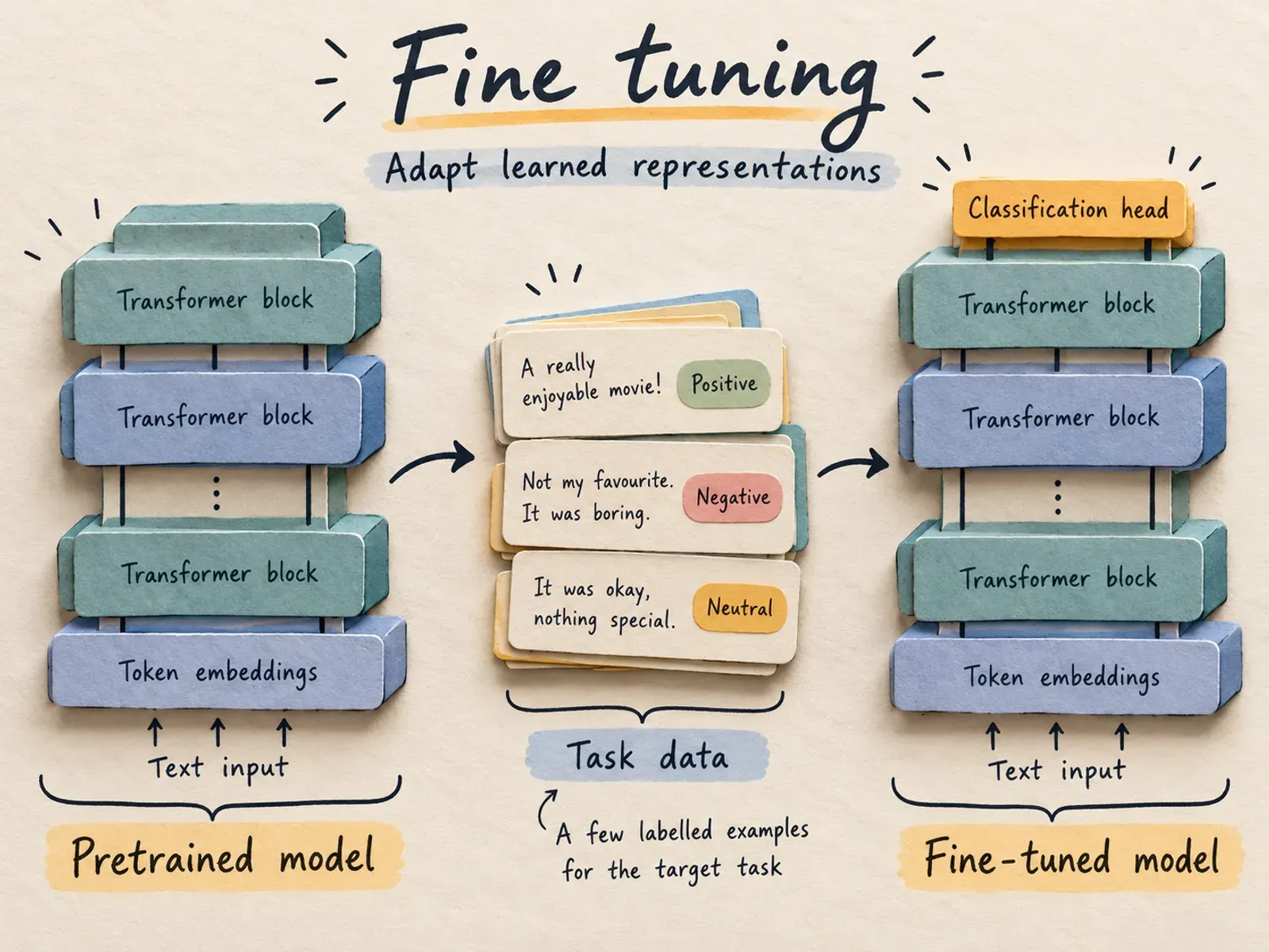
Fine-tuning means continuing training from a pretrained model so its parameters become more useful for a particular task or data distribution. For text classification, that usually means attaching a small prediction layer, showing the model labeled examples, and updating its weights using the errors it makes.
Text classification assigns an input to one of a predefined set of categories. A data distribution describes the patterns and frequencies of examples a model encounters. The opening illustration uses a few labeled examples as a visual shorthand for task adaptation; a useful model requires a sufficiently large, representative training and evaluation collection.
The difficult part is deciding what a successful update means. A model can improve its average score while missing most neutral tweets. It can score well on held-out news articles and misclassify a clearly written sports headline. Understanding those failures requires connecting the task, architecture, input representation, loss, and evaluation.
This article builds that connection in three stages: a numerical explanation of learning and metrics, a complete sentiment-classification workflow with DistilBERT, and a separate news-classification workflow with DistilGPT2. It then explains what changes when the output is a generated summary instead of a class label.
About the results: the recorded experiment tables describe earlier runs. The expanded teaching code below has not been run here to reproduce those experiments. Arithmetic examples are explicitly illustrative. Training time, learned probabilities, exact tokenized samples, and final scores depend on the environment, data revision, seed, and preprocessing; the recorded values are observations, not promised outputs.
What changes when we fine-tune a model?
Pretraining is the initial learning process that gives a model broadly useful representations from a large collection of examples. A representation is a vector of numbers that encodes features useful to the model. A parameter, also called a weight, is a learned numerical value inside the model.
An encoder such as BERT learns partly by recovering hidden tokens from their context. A causal language model such as GPT learns to predict the next token from the preceding tokens. Neither objective directly says, “Classify this tweet as negative, neutral, or positive.” Fine-tuning supplies that task-specific objective.
Large text collection → pretraining → pretrained weights
                                            ↓
Labeled task examples → task loss → updated task-specific weights
A label is the desired answer supplied with a training example. For a sentiment dataset, "The update fixed my problem" might have the label positive. The model predicts a label, compares its prediction with the supplied answer, and adjusts its parameters.
A classification head is the final trainable layer or small network that turns the model’s representation into one score per class. The backbone is the pretrained network beneath that head. The head usually starts with new random parameters when the checkpoint was pretrained for a different objective.
Full fine-tuning, frozen features, and adapters
Full fine-tuning allows all model parameters to change. Freezing a parameter means excluding it from gradient updates. An adapter is a small trainable addition to a larger model. Parameter-efficient fine-tuning, or PEFT, changes a relatively small set of parameters instead of updating the entire backbone.
LoRA, short for low-rank adaptation, learns a weight update using two smaller matrices. In the diagram, is a frozen weight matrix, and are trainable matrices, and is their matrix product.
For with shape , choose with shape and with shape . The rank setting limits how many independent directions the update can express and is chosen much smaller than either dimension. This reduces the trainable parameter count from to for that weight update. The diagram omits the configurable scale applied to . See the LoRA paper for the full method.
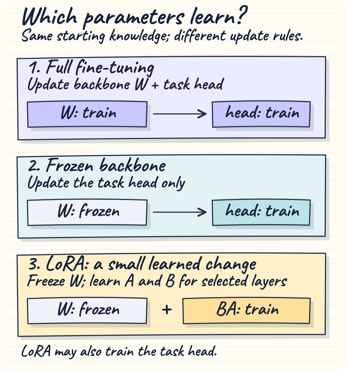
Choose which parameters can learn before comparing the cost or quality of two training methods.
| Method | What learns? | Practical consequence |
|---|---|---|
| Frozen backbone with a new head | The prediction head | A cheap baseline that tests the usefulness of existing features |
| Full fine-tuning | Backbone and head | Greater freedom to adapt, with more training memory and a risk of damaging useful pretrained behavior |
| LoRA | Small added low-rank matrices, plus any explicitly trainable task layers | Fewer trainable weights and optimizer states; the base model still has to be loaded and used |
Quantization stores numbers with fewer bits. QLoRA trains low-rank adapters through a frozen backbone stored in a 4-bit format; the QLoRA paper describes the additional memory-saving techniques. These methods are useful later, but they do not eliminate the need for clean data, a suitable objective, or an untouched test set.
The examples here use full fine-tuning. In attention layers, this includes the query, key, value, and output projection weights; it also includes feed-forward layers, normalization parameters, embeddings, and the new task head. Equal total and trainable parameter counts establish that weights are eligible for learning. They do not establish that every scalar changes on every update.
One parameter update, without hiding the symbols
A loss is a numerical penalty for a prediction. A gradient tells us how the loss changes when a trainable parameter changes. The learning rate sets the size of an update. An optimizer applies an update rule using those gradients.
Let denote a parameter value before update , the loss, and the learning rate. The simplest gradient-descent rule is:
For an illustrative single parameter, suppose , its gradient is , and . Then:
The positive gradient means increasing this parameter locally increases the loss; subtracting a small positive amount moves in the opposite direction. Real Transformer training uses millions of coupled parameters and an optimizer such as AdamW, which also tracks information from past gradients and applies weight decay. The simple equation explains the direction of learning, rather than every detail of AdamW.
Backpropagation computes gradients by applying the chain rule backward through the computation. It does not itself update the weights. That happens during the optimizer step.
Choose an architecture by its information flow
A Transformer is a neural network architecture built around attention and position-wise transformations. Attention mixes information between token representations by assigning different weights to other positions. A token is a text unit from the model’s vocabulary; it may be a word, a word fragment, or a byte-derived piece.
| Family | Examples | Information available at each position | Common uses |
|---|---|---|---|
| Encoder-only | BERT, DistilBERT, RoBERTa | Both earlier and later input tokens | Classification, entity extraction, extractive question answering |
| Decoder-only | GPT-2, DistilGPT2 | The current token and earlier tokens | Next-token prediction and text generation; also classification with a suitable head |
| Encoder–decoder | T5, FLAN-T5, BART, Pegasus | Encoder sees the source; decoder sees earlier output tokens and encoder states | Translation, summarization, other sequence-to-sequence tasks |
Bidirectional attention allows a token to use context on both sides. Causal attention prevents a token from reading later positions. Autoregressive generation repeatedly predicts a next token using the tokens available so far.
Consider “The bank approved the loan.” An encoder can use “loan” when building the representation of “bank.” A causal decoder’s representation at “bank” cannot use the later word “loan.” Its representation at the end of the sentence can, however, incorporate all preceding words. That is why a causal decoder can still classify a complete input.
What the attention mask actually changes
Inside one attention head, a query vector expresses what a position is looking for, a key vector expresses what another position offers, and a value vector carries the information to mix. A projection is a learned linear transformation that creates such vectors from hidden states.
Let , , and be the matrices containing these vectors, the key-vector width, and an additive mask. Scaled dot-product attention is:
Here is the transpose of . Softmax, defined numerically below, turns scores into weights. Allowed positions receive a mask value of zero; blocked positions receive a very large negative value, conceptually negative infinity, so their attention weights become zero.
                 Positions a token may read
Encoder                    Causal decoder
       1 2 3 4                    1 2 3 4
token1 ✓ ✓ ✓ ✓             token1 ✓ × × ×
token2 ✓ ✓ ✓ ✓             token2 ✓ ✓ × ×
token3 ✓ ✓ ✓ ✓             token3 ✓ ✓ ✓ ×
token4 ✓ ✓ ✓ ✓             token4 ✓ ✓ ✓ ✓
The causal mask and the padding mask solve different problems. The causal mask blocks future information. The padding mask blocks artificial filler positions. A GPT classifier needs correct handling of both.
Turn text into tensors without changing its meaning accidentally
Tokenization converts text into vocabulary pieces and their integer IDs. An embedding maps each ID to a learned vector. A tensor is a multidimensional array; a batch of token IDs usually has shape [batch_size, sequence_length].
Always start with the tokenizer that belongs to the pretrained checkpoint. An ID is an address into that checkpoint’s embedding table. An arbitrary replacement tokenizer can give that address a different meaning.
BERT-style special tokens
A special token is a reserved symbol used to mark structure rather than an ordinary text fragment.
[CLS] I really enjoyed this movie [SEP] [PAD] [PAD]
  ↑                                      ↑
sequence start artificial filler| Symbol | Purpose |
|---|---|
[CLS] | A special first position whose final representation can feed a sequence classifier |
[SEP] | A separator or boundary marker |
[PAD] | Filler used to make tensors compatible in a batch |
[MASK] | A marker for hidden tokens in masked-language-model pretraining |
[UNK] | A fallback for text the tokenizer cannot represent with its ordinary pieces |
[CLS] does not inherently mean “the sentiment of this sentence.” Its usefulness as a classification representation depends on the architecture and training. DistilBERT’s sequence-classification head transforms the hidden state at the first position and maps it to class scores.
An uncased tokenizer normalizes capitalization; a cased tokenizer preserves relevant case distinctions. Losing case can remove useful signals for named entity recognition, the task of finding names such as people or locations in text. An uncased model can still learn entity recognition; it simply cannot use the original capitalization signal in the same way.
Padding, truncation, and the input attention mask
Padding adds filler positions so examples can share one rectangular tensor. Truncation removes tokens beyond a chosen limit. The attention mask marks real input positions with 1 and padding with 0 in the tokenizer output.
Illustrative BERT token IDs:
input_ids:       101 2023 2003 2204 102   0   0
attention_mask:    1    1    1    1   1   0   0
An attention mask is not a class label, a confidence value, or a mechanism for restoring truncated text. Once the end of a review is truncated, a final sentence such as “Actually, I would never buy this again” may be missing entirely.
Static padding pads every example to a fixed length. Dynamic padding pads each batch only to its longest example. Static padding is easy to inspect; dynamic padding often avoids wasted work. The classification examples below use fixed length 128 so their input shapes are explicit.
For ordinary dense attention, the attention-score matrix has approximately entries per head for sequence length . Moving from 128 to 256 tokens makes that matrix four times as large. The whole model’s time and memory do not necessarily increase by exactly four times, because other operations and implementation choices also matter.
Measure token lengths before selecting the limit. Report the fraction that exceed the cap using untruncated lengths. A processed example of length 128 might originally have had exactly 128 tokens or many more; the capped length alone cannot tell you.
Separate learning, model selection, and final evaluation
The training set provides examples used for parameter updates. The validation set guides development choices. The test set estimates final performance on data withheld from those choices. A split is one of these separate dataset partitions.
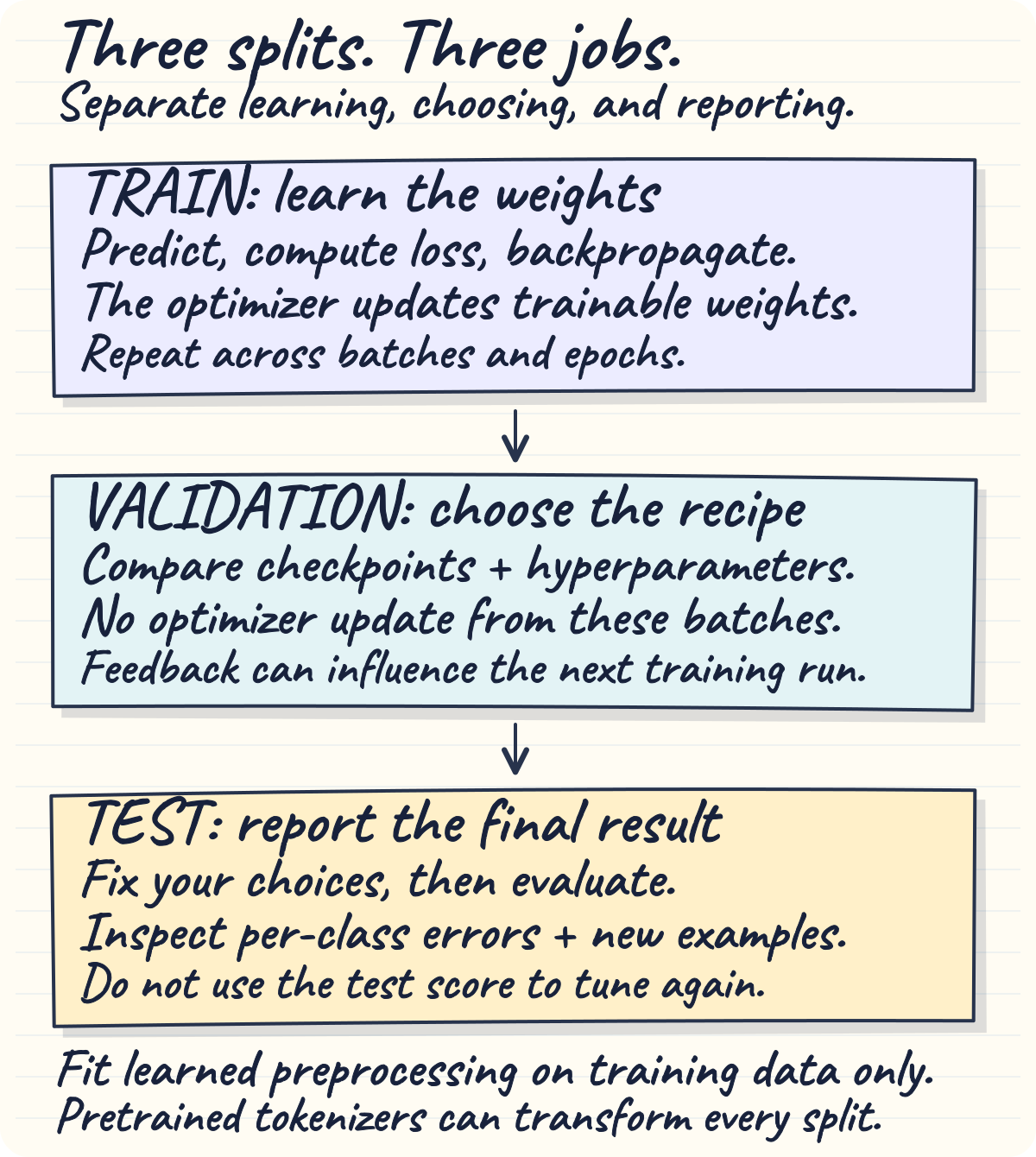
Validation participates in development decisions. The test set is reserved for evaluating the chosen procedure.
A hyperparameter is a setting chosen outside the weight-learning process, such as learning rate, batch size, or number of epochs. An epoch is one pass through the training examples. A checkpoint is a saved model state, often including enough information to resume training.
Selecting the best validation checkpoint is legitimate. Selecting the learning rate by repeatedly checking the test score turns the test set into another development set. A fresh holdout is then needed for an honest final estimate.
An unseen example should also be independent enough for the intended evaluation. Different rows containing the same tweet, near-duplicate headlines, or texts by the same source can cross split boundaries. For production forecasting, a chronological split may be more informative than a random one. A data leak occurs when information that should be unavailable during development influences training or selection.
The word “test” does not guarantee an unbiased result. Independence, representative sampling, label quality, and disciplined model selection are the conditions that make the result useful.
Follow one classification prediction into its loss
Logits are raw, unrestricted class scores produced before converting them into probabilities. Softmax converts a vector of scores into positive numbers that sum to one. Cross-entropy penalizes assigning too little probability to the correct label.
Suppose the class order is [negative, neutral, positive], and a model produces the illustrative logits:
z = [0.0, 1.0, 2.0]
true label = positive, index 2
For class , with score , softmax is:
The exponentials are approximately . Their sum is , giving:
negative: 0.0900
neutral:  0.2447
positive: 0.6652
Argmax returns the index of the largest value, so the predicted label is positive. The cross-entropy for correct class is:
Here is the natural logarithm. For a positive label, . If the same input were actually negative, the loss would be . The model receives a larger penalty for putting little probability on the supplied correct answer.
The following is an independent arithmetic example, with no pretrained model or training required:
import torch

logits = torch.tensor([[0.0, 1.0, 2.0]], requires_grad=True)
labels = torch.tensor([2])
probabilities = torch.softmax(logits, dim=-1)
loss = torch.nn.functional.cross_entropy(logits, labels)
loss.backward()

print(probabilities.detach().round(decimals=4))
print(round(loss.item(), 4))
print(logits.grad.round(decimals=4))
Expected arithmetic output, subject to display formatting:
tensor([[0.0900, 0.2447, 0.6652]])
0.4076
tensor([[ 0.0900,  0.2447, -0.3348]])
The negative gradient on the correct class encourages its logit to increase. Positive gradients on competing classes encourage their logits to decrease. These gradients flow backward into the head and, during full fine-tuning, into the backbone.
Pass raw logits to PyTorch’s classification cross-entropy function. Applying softmax first changes the input the loss function expects; the function already handles the required log-softmax operation internally. See PyTorch’s CrossEntropyLoss contract.
The practical loop is therefore: construct a batch, run the forward computation, obtain logits and loss, backpropagate the loss, apply the optimizer update, and clear gradients before the next independent update. Trainer coordinates these operations for us.
Understand accuracy, precision, recall, and F1 before reporting them
Accuracy is the fraction of all examples classified correctly. Precision asks what fraction of predictions for a chosen class are correct. Recall asks what fraction of actual members of that class the model finds. F1 is the harmonic mean of precision and recall, rewarding a balance between the two.
For a chosen positive class, a true positive (TP) is a correctly predicted positive, a false positive (FP) is a negative example predicted positive, a false negative (FN) is a positive example missed, and a true negative (TN) is a correctly predicted negative. Support is the number of actual examples belonging to a class.
A confusion matrix counts predictions against actual labels. Its row and column meanings must always be stated.
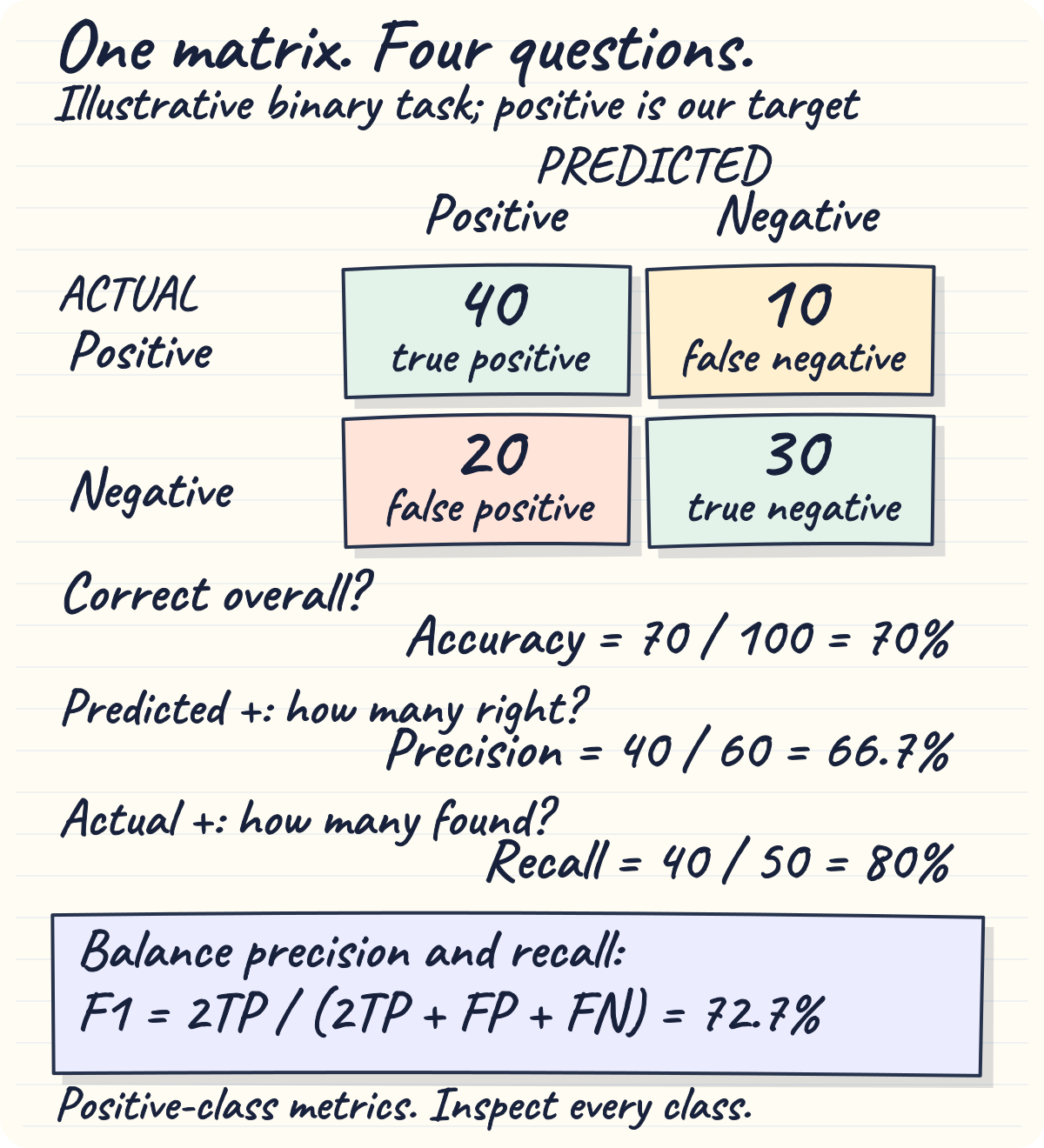
These illustrative counts demonstrate why four metrics can describe the same predictions differently.
There are 100 examples: 50 actual positives and 50 actual negatives. The model predicts positive 60 times, getting 40 of those predictions right.
“The model finds 80% of positives” describes recall. It does not mean 80% of its positive predictions are reliable; their precision is about 66.7%.
For multiple classes, calculate these quantities for each class by treating it as the chosen positive class and grouping all others together. Macro F1 averages class F1 scores equally. Weighted F1 averages them in proportion to their supports. Macro F1 gives a rare class the same importance as a frequent one; weighted F1 reflects class frequency in the evaluation set. Neither is a substitute for examining individual classes.
For example, if class F1 values are with supports , macro F1 is , while weighted F1 is . The larger weighted result can coexist with poor performance on the smaller class. The averaging definitions are documented in scikit-learn’s metric reference.
Some metrics are undefined when their denominator is zero. In the code below, zero_division=0 makes that convention explicit. Also inspect whether a class received any predictions; a zero score can reveal a model that has ignored it entirely.
The right precision–recall balance depends on error costs. Missing an urgent message and incorrectly flagging a harmless message can have different consequences. A decision threshold is the score cutoff used to choose a class. It can be adjusted using validation data for a binary classifier when the deployment requirement calls for it, but the threshold and its costs must be evaluated on representative data.
Prepare a reproducible training environment
The main examples assume Python, a working PyTorch installation for your device, internet access for public model and dataset downloads, and enough disk space for caches and checkpoints. A supported GPU can make full fine-tuning much faster; the code does not require one or enable mixed precision blindly.
Install PyTorch using the command appropriate for your operating system and accelerator, then install the libraries used here:
python -m pip install transformers datasets accelerate scikit-learn numpy sentencepieceHugging Face Transformers provides model and tokenizer interfaces. Datasets loads and transforms dataset splits. Accelerate supplies device and distributed-training support used by Trainer. scikit-learn supplies the metrics in these examples. SentencePiece supports the T5 tokenizer used in the final teaching example.
The API pattern uses eval_strategy in TrainingArguments and processing_class in Trainer, consistent with the current classification guide. Record the versions you actually use and keep a dependency lock for a repeatable experiment. An unpinned install command cannot promise bitwise reproduction over time.
The following blocks form the shared setup and then a complete sentiment workflow. The news example explicitly creates its own data, model, and trainer; it reuses only shared imports and helper functions.
import math
from collections import Counter
from importlib.metadata import version
from pathlib import Path

import numpy as np
import torch
from datasets import Dataset, DatasetDict, load_dataset
from sklearn.metrics import (
    accuracy_score,
    classification_report,
    confusion_matrix,
    f1_score,
)
from transformers import (
    AutoModelForSequenceClassification,
    AutoModelForSeq2SeqLM,
    AutoTokenizer,
    DataCollatorForSeq2Seq,
    DataCollatorWithPadding,
    Seq2SeqTrainer,
    Seq2SeqTrainingArguments,
    Trainer,
    TrainingArguments,
    set_seed,
)

SEED = 42
set_seed(SEED)

for package in ["torch", "transformers", "datasets", "accelerate", "scikit-learn"]:
    print(f"{package}: {version(package)}")
print("CUDA available:", torch.cuda.is_available())
A seed initializes random-number generators so an experiment is easier to repeat. It does not eliminate every source of nondeterminism across hardware, libraries, or parallel execution. CUDA availability is only one accelerator check; False does not establish that every possible hardware backend is unavailable.
The two classifiers use the same metric function. No softmax is needed to find the winning class: it preserves the ordering of logits.
def compute_classification_metrics(eval_prediction):
    logits, labels = eval_prediction
    if isinstance(logits, tuple):
        logits = logits[0]
    predictions = np.argmax(logits, axis=-1)
    return {
        "accuracy": float(accuracy_score(labels, predictions)),
        "f1_weighted": float(
            f1_score(labels, predictions, average="weighted", zero_division=0)
        ),
        "f1_macro": float(
            f1_score(labels, predictions, average="macro", zero_division=0)
        ),
    }


def print_parameter_counts(model):
    total = sum(parameter.numel() for parameter in model.parameters())
    trainable = sum(
        parameter.numel()
        for parameter in model.parameters()
        if parameter.requires_grad
    )
    print(f"Total parameters: {total:,}")
    print(f"Trainable parameters: {trainable:,}")
    print(f"FP32 parameter storage only: {total * 4 / 1_000_000:.1f} MB")


def print_classification_details(prediction_output, label_names):
    logits = prediction_output.predictions
    if isinstance(logits, tuple):
        logits = logits[0]
    predictions = np.argmax(logits, axis=-1)
    labels = prediction_output.label_ids
    class_ids = list(range(len(label_names)))
    print(classification_report(
        labels,
        predictions,
        labels=class_ids,
        target_names=label_names,
        digits=4,
        zero_division=0,
    ))
    print("Confusion matrix: actual rows, predicted columns")
    print(confusion_matrix(labels, predictions, labels=class_ids))
FP32 stores each floating-point parameter in 32 bits, or four bytes. Activations are intermediate values produced as an input passes through the network. Parameter storage is only part of training memory. Gradients, optimizer state, activations retained for backpropagation, temporary workspaces, and framework overhead also require memory. A 268 MB weight estimate is not a 268 MB training-memory estimate.
Experiment 1: fine-tune DistilBERT for tweet sentiment
DistilBERT is a smaller BERT-style encoder trained using knowledge distillation, a process in which a smaller model learns from a larger model’s behavior as well as training objectives. We will use its uncased checkpoint with a three-class sentiment head.
The task is to map an English tweet to negative, neutral, or positive. The dataset card describes the multilingual source and its language subsets; read its provenance and usage conditions before reusing it in a product.
Load splits and inspect the labels
SENTIMENT_MODEL = "distilbert/distilbert-base-uncased"
SENTIMENT_LABELS = ["negative", "neutral", "positive"]
SENTIMENT_MAX_LENGTH = 128
SENTIMENT_BATCH_SIZE = 32

sentiment_data = load_dataset(
    "cardiffnlp/tweet_sentiment_multilingual",
    revision="refs/convert/parquet",
    data_dir="english",
)

for split_name, split in sentiment_data.items():
    counts = Counter(split["label"])
    print(split_name, len(split), dict(sorted(counts.items())))

feature = sentiment_data["train"].features["label"]
print("Dataset label names:", feature.names)
assert list(feature.names) == SENTIMENT_LABELS
assert set(sentiment_data) == {"train", "validation", "test"}
The explicit Parquet revision selects a data-only representation rather than relying on an older executable loading script. A revision identifies a branch, tag, or commit of a repository. This conversion branch is not an immutable experiment lock; for strict reproduction, record resolved dataset and model commit identifiers along with the dependency versions.
Recorded split sizes and class counts:
| Split | Examples | Negative | Neutral | Positive |
|---|---|---|---|---|
| Training | 1,839 | 613 | 613 | 613 |
| Validation | 324 | — | — | — |
| Test | 870 | 290 | 290 | 290 |
The validation class counts are deliberately left unspecified here; print them from the data you load. The equal training counts matter: if neutral sentiment is difficult later, fewer neutral training examples cannot explain that result. Balance does not make labels unambiguous or linguistic patterns equally easy.
Tokenize every split with one policy
sentiment_tokenizer = AutoTokenizer.from_pretrained(SENTIMENT_MODEL)


def tokenize_sentiment(batch):
    return sentiment_tokenizer(
        batch["text"],
        padding="max_length",
        truncation=True,
        max_length=SENTIMENT_MAX_LENGTH,
    )


sentiment_tokens = sentiment_data.map(tokenize_sentiment, batched=True)
sentiment_tokens = sentiment_tokens.remove_columns(["text"])
sentiment_tokens = sentiment_tokens.rename_column("label", "labels")
sentiment_tokens.set_format("torch")

sample = sentiment_tokens["train"][0]
print("Vocabulary:", sentiment_tokenizer.vocab_size)
print("Input shape:", sample["input_ids"].shape)
print("Mask shape:", sample["attention_mask"].shape)
print("First IDs:", sample["input_ids"][:10].tolist())
print("Real token count:", int(sample["attention_mask"].sum()))
Recorded tokenization inspection:
Vocabulary: 30522
Input shape: torch.Size([128])
Mask shape: torch.Size([128])
First IDs: [101, 3100, 1045, 1032, 23343, 24096, 2683, 2213, 3374, 2021]
The vocabulary contains 30,522 entries. ID 101 is the [CLS] marker for this checkpoint. A single example has shape [128]; a batch of 32 examples has shape [32, 128]. The associated labels tensor contains one integer per example, giving shape [32] for a full batch.
Renaming the target to labels makes the model’s training interface explicit. Passing labels to the sequence-classification model lets it calculate the task loss. set_format("torch") requests PyTorch tensors when examples are retrieved.
Attach the new head and check what is trainable
set_seed(SEED)
sentiment_model = AutoModelForSequenceClassification.from_pretrained(
    SENTIMENT_MODEL,
    num_labels=len(SENTIMENT_LABELS),
    id2label={index: label for index, label in enumerate(SENTIMENT_LABELS)},
    label2id={label: index for index, label in enumerate(SENTIMENT_LABELS)},
)
print_parameter_counts(sentiment_model)
Recorded parameter inspection:
Total parameters: 66,955,779
Trainable parameters: 66,955,779
FP32 parameter storage only: 267.8 MB
A warning that classification-head parameters were newly initialized is expected when loading a general pretrained checkpoint into this task-specific model. It means the head still needs training. Warnings about incompatible dimensions or unexpectedly missing backbone weights need separate investigation.
Configure training and validation
Batch size is the number of examples processed together. A training step usually refers to a parameter update; gradient accumulation, explained later, can combine several batches into one such update. Weight decay discourages large parameter values through the optimizer’s regularization rule. Regularization means a technique intended to reduce overfitting, where a model fits training examples better than it generalizes to new ones.
sentiment_arguments = TrainingArguments(
    output_dir="./runs/sentiment-distilbert",
    learning_rate=2e-5,
    per_device_train_batch_size=SENTIMENT_BATCH_SIZE,
    per_device_eval_batch_size=32,
    num_train_epochs=3,
    weight_decay=0.01,
    eval_strategy="epoch",
    save_strategy="epoch",
    load_best_model_at_end=True,
    metric_for_best_model="f1_weighted",
    greater_is_better=True,
    save_total_limit=2,
    report_to="none",
    seed=SEED,
    data_seed=SEED,
)

sentiment_trainer = Trainer(
    model=sentiment_model,
    args=sentiment_arguments,
    train_dataset=sentiment_tokens["train"],
    eval_dataset=sentiment_tokens["validation"],
    processing_class=sentiment_tokenizer,
    data_collator=DataCollatorWithPadding(sentiment_tokenizer),
    compute_metrics=compute_classification_metrics,
)

print("Single-device batches per epoch:", math.ceil(
    len(sentiment_tokens["train"]) / SENTIMENT_BATCH_SIZE
))
The single-device, no-accumulation calculation gives batches per epoch when the incomplete final batch is retained. Integer floor division gives 57 full batches and misses the last 15 examples. Distributed sampling or different loader options can change the actual count.
TrainingArguments declares the training policy; Trainer connects that policy to a particular model and datasets. A newly created model does not replace the model inside an existing trainer automatically. Creating an explicit trainer for each experiment prevents a subtle and expensive mistake: training the previous task again.
The chosen learning rate, , is a reasonable starting candidate rather than a universal optimum. Three epochs limit this initial experiment; they do not guarantee the absence of overfitting. The sequence limit controls information retention, and the batch size controls both memory and the update statistics.
At the end of every epoch, this configuration validates and saves a checkpoint. load_best_model_at_end=True restores the saved checkpoint with the highest validation weighted F1. It does not necessarily restore the final epoch. Early stopping is a separate policy that ends training after the validation metric fails to improve for a chosen patience, the number of evaluation checks allowed without sufficient improvement. Simply restoring the best checkpoint does not turn early stopping on. The Trainer reference defines these controls.
Train, then evaluate the selected model
The next block performs the actual training when you run it. It downloads weights and uses your local compute; the printed results must come from that run.
sentiment_training_result = sentiment_trainer.train()
print(sentiment_training_result.metrics)

sentiment_test_output = sentiment_trainer.predict(
    sentiment_tokens["test"], metric_key_prefix="test"
)
print(sentiment_test_output.metrics)
print_classification_details(sentiment_test_output, SENTIMENT_LABELS)
Using predict returns the metrics and prediction logits from the same test pass, which lets us inspect class behavior without a second prediction pass. Keep this final test evaluation separate from hyperparameter selection.
Recorded training summary:
| Measurement | Recorded value |
|---|---|
| Training runtime | 141.8040 seconds |
| Training examples per second | 38.9060 |
| Optimizer steps per second | 1.2270 |
| Reported training loss | 0.8273 |
| Completed epochs | 3 |
Recorded held-out test summary:
| Measurement | Recorded value |
|---|---|
| Loss | 0.7470 |
| Accuracy | 0.6598 |
| Weighted F1 | 0.6493 |
| Macro F1 | 0.6493 |
The training loss is an aggregate reported across training updates, not necessarily the loss of the restored best checkpoint measured afterward. Training and evaluation also differ in behaviors such as dropout, so comparing those two scalar losses alone is not a full generalization diagnosis.
Dropout randomly suppresses selected activations during training as a regularizer. Evaluation mode disables that random suppression. Runtime and throughput are particular to the recorded environment and should not be used to size a different machine.
The neutral class changes the interpretation
| Class | Precision | Recall | F1 | Support |
|---|---|---|---|---|
| Negative | 0.62 | 0.89 | 0.73 | 290 |
| Neutral | 0.57 | 0.43 | 0.49 | 290 |
| Positive | 0.80 | 0.66 | 0.73 | 290 |
These recorded class metrics are rounded. A neutral recall of 0.43 means the model recognizes only about 43% of actual neutral examples. Roughly 57% are assigned another sentiment. It does not mean that 43% of neutral predictions are correct; that would describe precision.
Neutral examples may lack overt emotion, contain mixed sentiment, or depend on conversational context. Those are hypotheses to test by reading errors, rather than conclusions established by this table. Start with the confusion matrix, inspect the neutral-to-negative and neutral-to-positive pairs, and examine whether annotators would agree on the intended label.
Macro and weighted F1 match because the test supports are equal. That equality is arithmetic, not evidence that all classes behave similarly. A model that always picks one of three equally frequent classes has accuracy about 33.3%; the observed 66% is above that trivial baseline, but its suitability still depends on the application’s requirements and stronger baselines.
Inference: make device placement and label mapping explicit
Inference means using a trained model to produce predictions without updating its weights.
Inference means using trained weights to make predictions without updating them. The helper below works for either classifier in this article. It returns the chosen label and the full score distribution, so an ambiguous prediction remains inspectable.
def predict_text(model, tokenizer, text, max_length=128):
    if not isinstance(text, str) or not text.strip():
        raise ValueError("Provide a non-empty string.")

    encoded = tokenizer(
        text,
        return_tensors="pt",
        truncation=True,
        max_length=max_length,
    )
    device = next(model.parameters()).device
    encoded = {name: tensor.to(device) for name, tensor in encoded.items()}

    model.eval()
    with torch.inference_mode():
        logits = model(**encoded).logits
        probabilities = torch.softmax(logits, dim=-1)[0]

    predicted_id = int(probabilities.argmax().item())
    scores = {
        model.config.id2label[index]: float(probabilities[index].item())
        for index in range(probabilities.numel())
    }
    return {
        "label": model.config.id2label[predicted_id],
        "score": scores[model.config.id2label[predicted_id]],
        "all_scores": scores,
    }


for text in [
    "I absolutely love this product! Best purchase ever!",
    "Not impressed. Expected much better quality.",
]:
    print(predict_text(
        sentiment_trainer.model,
        sentiment_tokenizer,
        text,
        max_length=SENTIMENT_MAX_LENGTH,
    ))
Trainer may have moved the model onto a GPU. The tokenizer creates CPU tensors by default, so moving them to the model’s device avoids a device mismatch. This helper assumes a normal single-device model, as used here; a sharded deployment needs its own device-management strategy.
Recorded predictions for those two sentences:
| Input | Predicted class | Largest softmax score |
|---|---|---|
| “I absolutely love this product! Best purchase ever!” | Positive | 0.810 |
| “Not impressed. Expected much better quality.” | Positive | 0.433 |
The second prediction conflicts with the clear negative meaning of the sentence. Its 0.433 score is also below 0.5; in a three-class problem a winning score need not exceed 0.5. Calibration describes how closely predicted probabilities correspond to observed correctness rates. A softmax score is not automatically a calibrated probability of being correct.
Save the complete inference package
sentiment_export = Path("./exports/sentiment-distilbert")
sentiment_trainer.save_model(str(sentiment_export))
sentiment_tokenizer.save_pretrained(str(sentiment_export))

# Later, in a fresh process with the same dependencies:
reloaded_tokenizer = AutoTokenizer.from_pretrained(str(sentiment_export))
reloaded_model = AutoModelForSequenceClassification.from_pretrained(
    str(sentiment_export)
)
print(predict_text(reloaded_model, reloaded_tokenizer, "The service was fine."))
Save the tokenizer, model configuration, label mapping, preprocessing policy, and evaluation record together. Saving only a weight tensor leaves important parts of the input/output contract unspecified. Resuming the optimizer from a training checkpoint is a different operation from loading an inference package.
Experiment 2: adapt a causal decoder for news classification
DistilGPT2 is a smaller GPT-2-style causal decoder. We will attach a four-class sequence-classification head to it. This is supervised classification using a decoder backbone; it is not a text-generation prompt asking the model to spell a category name.
The AG News dataset has 120,000 training examples and 7,600 test examples across World, Sports, Business, and Sci/Tech. The teaching experiment uses smaller subsets: 2,400 training, 400 validation, and 1,000 test examples.
Build disjoint subsets explicitly
Stratification preserves chosen class proportions when constructing a subset or split. We select 700 examples per class from the source training partition, then split them into 600 training and 100 validation examples per class. The test subset comes only from the source test partition.
NEWS_MODEL = "distilbert/distilgpt2"
NEWS_LABELS = ["World", "Sports", "Business", "Sci/Tech"]
NEWS_MAX_LENGTH = 128

news_source = load_dataset("fancyzhx/ag_news")
assert list(news_source["train"].features["label"].names) == NEWS_LABELS


def balanced_subset(split, per_class, seed):
    labels = np.asarray(split["label"])
    random_generator = np.random.default_rng(seed)
    chosen_indices = []
    for class_id in range(len(NEWS_LABELS)):
        candidates = np.flatnonzero(labels == class_id)
        if len(candidates) < per_class:
            raise ValueError(f"Not enough examples for class {class_id}")
        chosen_indices.extend(random_generator.choice(
            candidates, size=per_class, replace=False
        ).tolist())
    random_generator.shuffle(chosen_indices)
    return split.select(chosen_indices)


news_development = balanced_subset(news_source["train"], 700, SEED)
news_split = news_development.train_test_split(
    test_size=400,
    stratify_by_column="label",
    seed=SEED,
)
news_data = DatasetDict({
    "train": news_split["train"],
    "validation": news_split["test"],
    "test": balanced_subset(news_source["test"], 250, SEED),
})

for split_name, split in news_data.items():
    print(split_name, len(split), dict(sorted(Counter(split["label"]).items())))
Expected subset sizes from this construction:
train 2400 {0: 600, 1: 600, 2: 600, 3: 600}
validation 400 {0: 100, 1: 100, 2: 100, 3: 100}
test 1000 {0: 250, 1: 250, 2: 250, 3: 250}
This is an explicit new subset-construction policy. Matching the number of examples in an earlier experiment does not establish that the selected rows, random seed, or results match it. The class prior is the frequency of a class before considering an input’s features. Balanced test sampling also changes that prior relative to a production stream; retain natural-frequency evaluation when that is the relevant deployment question.
Fix GPT-2 padding without changing token positions unnecessarily
GPT-2’s tokenizer has no dedicated padding token by default. An end-of-sequence token, or EOS token, marks a sequence boundary in conventions that use it. We can reuse it as the filler ID, provided the attention mask marks actual padding and the model configuration knows the selected padding ID.
news_tokenizer = AutoTokenizer.from_pretrained(NEWS_MODEL)
print("Default padding token:", news_tokenizer.pad_token)

news_tokenizer.pad_token = news_tokenizer.eos_token
news_tokenizer.padding_side = "right"

print("Padding token ID:", news_tokenizer.pad_token_id)
print("EOS token ID:", news_tokenizer.eos_token_id)
Expected configuration for this checkpoint:
Default padding token: None
Padding token ID: 50256
EOS token ID: 50256
Position embeddings provide information about token order. GPT-2 uses learned absolute position embeddings. Right padding preserves a real token’s position index regardless of how much padding follows it. The GPT-2 documentation recommends right padding for this reason and explains that its sequence classifier uses the last non-padding token when a padding ID is configured.
Real content: The market rallied today
Right padding: The market rallied today PAD PAD PAD
                                      ↑
                    classifier uses the last non-PAD position
The historical decoder experiment used left padding. Its inspected sample began with ten 50256 IDs and ten zero mask values, had 68 padding positions, and ended with a real-token mask value of 1. That illustrates how padding IDs and masks relate. It is not a requirement that every GPT classifier use left padding.
If you deliberately left-pad GPT-2 during a direct forward pass, verify the position_ids policy: a padding mask alone does not necessarily renumber absolute positions. Generation libraries may implement different position handling, so a generation recommendation should not be copied into a classification experiment without checking the model path.
Reusing EOS as PAD does not mean the tokenizer automatically appends EOS to every text. The default GPT-2 tokenizer does not do that. These examples classify ordinary text without explicitly inserted EOS markers. If real EOS tokens must occur inside inputs, a separate PAD token and resized embeddings may be a better contract because padding-ID-based pooling otherwise treats those IDs as filler.
Inspect lengths before truncation
def news_token_lengths(batch):
    encoded = news_tokenizer(batch["text"], truncation=False)
    return {"token_length": [len(ids) for ids in encoded["input_ids"]]}


news_lengths = news_data["train"].map(news_token_lengths, batched=True)
lengths = np.asarray(news_lengths["token_length"])
print("Median tokens:", float(np.median(lengths)))
print("Examples exceeding the cap:", int((lengths > NEWS_MAX_LENGTH).sum()))
print("Fraction exceeding the cap:", float((lengths > NEWS_MAX_LENGTH).mean()))
Recorded length observations were a median of 50 tokens and 12 examples, or 0.5% of 2,400, reaching the 128-token cap. They suggest that 128 was a plausible compromise for that subset, but “reaching the cap” is weaker evidence than measuring original lengths. The code above measures actual exceedances. Neither statistic proves that the discarded information is irrelevant to the label.
Tokenize and create a separate decoder model
def tokenize_news(batch):
    return news_tokenizer(
        batch["text"],
        padding="max_length",
        truncation=True,
        max_length=NEWS_MAX_LENGTH,
    )


news_tokens = news_data.map(tokenize_news, batched=True)
news_tokens = news_tokens.remove_columns(["text"])
news_tokens = news_tokens.rename_column("label", "labels")
news_tokens.set_format("torch")

set_seed(SEED)
news_model = AutoModelForSequenceClassification.from_pretrained(
    NEWS_MODEL,
    num_labels=len(NEWS_LABELS),
    id2label={index: label for index, label in enumerate(NEWS_LABELS)},
    label2id={label: index for index, label in enumerate(NEWS_LABELS)},
)
news_model.config.pad_token_id = news_tokenizer.pad_token_id
print_parameter_counts(news_model)
Recorded parameter inspection:
Total parameters: 81,915,648
Trainable parameters: 81,915,648
FP32 parameter storage only: 327.7 MB
The new score head maps a token representation to four class scores. At a real final token, causal attention has had access to the preceding input, making that position usable for sequence classification. The head’s weights need training, and pad_token_id must agree between tokenizer and model.
Compared with the sentiment model, this decoder has more parameters, but parameter count alone does not determine memory or speed. The news experiment uses a smaller device batch of 16 as a practical starting point.
Train with its own arguments and trainer
news_arguments = TrainingArguments(
    output_dir="./runs/news-distilgpt2",
    learning_rate=2e-5,
    per_device_train_batch_size=16,
    per_device_eval_batch_size=16,
    num_train_epochs=3,
    weight_decay=0.01,
    eval_strategy="epoch",
    save_strategy="epoch",
    load_best_model_at_end=True,
    metric_for_best_model="f1_weighted",
    greater_is_better=True,
    save_total_limit=2,
    report_to="none",
    seed=SEED,
    data_seed=SEED,
)

news_trainer = Trainer(
    model=news_model,
    args=news_arguments,
    train_dataset=news_tokens["train"],
    eval_dataset=news_tokens["validation"],
    processing_class=news_tokenizer,
    data_collator=DataCollatorWithPadding(news_tokenizer),
    compute_metrics=compute_classification_metrics,
)

news_training_result = news_trainer.train()
print(news_training_result.metrics)
news_test_output = news_trainer.predict(news_tokens["test"], metric_key_prefix="test")
print(news_test_output.metrics)
print_classification_details(news_test_output, NEWS_LABELS)
Recorded training summary:
| Measurement | Recorded value |
|---|---|
| Training runtime | 211.7052 seconds |
| Training examples per second | 34.0100 |
| Reported training loss | 0.5998 |
| Completed epochs | 3 |
Recorded validation trend:
| Epoch | Loss | Accuracy | Weighted F1 | Macro F1 |
|---|---|---|---|---|
| 1 | 0.4915 | 0.8300 | 0.8288 | 0.8282 |
| 2 | 0.4087 | 0.8650 | 0.8642 | 0.8636 |
| 3 | 0.3754 | 0.8775 | 0.8769 | 0.8763 |
Lower validation loss and improving F1 across these three epochs are encouraging. They do not establish that additional epochs would continue to help. A single seed also cannot show how sensitive the result is to head initialization or subset selection.
Read the held-out result and its limitations
Recorded test summary:
| Measurement | Recorded value |
|---|---|
| Loss | 0.2710 |
| Accuracy | 0.8980 |
| Weighted F1 | 0.8982 |
| Macro F1 | 0.8984 |
Recorded class metrics:
| Class | Precision | Recall | F1 |
|---|---|---|---|
| World | 0.91 | 0.90 | 0.91 |
| Sports | 0.97 | 0.96 | 0.96 |
| Business | 0.85 | 0.86 | 0.86 |
| Sci/Tech | 0.87 | 0.87 | 0.87 |
The more precise class hit rates recorded were World 90.20%, Sports 96.00%, Business 86.38%, and Sci/Tech 86.69%. A hit rate among actual members of one class is recall, rather than a distinct form of overall accuracy. The class metrics above are rounded; full counts and a confusion matrix would be needed to reconstruct every aggregate exactly.
The recorded macro and weighted F1 differ slightly. On the newly constructed exactly balanced test subset, those two averages should be equal apart from negligible numerical effects. The differing recorded values are another reason not to assume that the new subset policy recreates the earlier test rows or class supports.
Four custom headlines are useful probes, not a new benchmark
An error probe is a deliberately chosen example that checks a particular behavior. Distribution shift means the relationship between deployment data and training or evaluation data has changed in a relevant way. Out-of-distribution data falls outside the patterns represented by the data used to develop the model.
news_probes = [
    (
        "UN Security Council holds emergency session over escalating tensions in the Middle East",
        "World",
    ),
    (
        "Manchester United defeat Liverpool 3-1 in dramatic Premier League showdown",
        "Sports",
    ),
    (
        "Federal Reserve raises interest rates by 25 basis points amid inflation concerns",
        "Business",
    ),
    (
        "NASA's Artemis mission successfully deploys new lunar surface habitat module",
        "Sci/Tech",
    ),
]

for headline, expected_label in news_probes:
    result = predict_text(news_trainer.model, news_tokenizer, headline, NEWS_MAX_LENGTH)
    print({"expected": expected_label, **result})
These are classification examples, not factual reporting that the described events happened. Recorded predictions were:
| Expected | Predicted | Largest softmax score |
|---|---|---|
| World | World | 0.572 |
| Sports | World | 0.694 |
| Business | World | 0.577 |
| Sci/Tech | Sci/Tech | 0.550 |
Only two of four probes were correct. This establishes failures on those sentences. It does not establish a 50% production accuracy, prove distribution shift, or rule out a preprocessing bug. Four hand-written examples are too small and selectively chosen to estimate a deployment rate.
First verify label order, tokenizer/model pairing, padding, position handling, truncation, and which checkpoint was loaded. Then collect a larger independent sample of recent domain text, label it consistently, and compare errors with the benchmark errors. A shift in vocabulary, style, article length, time period, or class frequencies may help explain the discrepancy after implementation mistakes have been excluded.
The sports error also illustrates why model score and correctness must be checked separately: a wrong answer can receive a larger softmax score than a correct answer on another example.
Why 90% versus 66% does not rank GPT above BERT
The two recorded experiments used different tasks, data, label definitions, and sample sizes. One separated news topics; the other separated sentiment in tweets. Their scores answer different questions.
| Property | DistilBERT experiment | DistilGPT2 experiment |
|---|---|---|
| Architecture | Encoder | Decoder |
| Attention | Bidirectional | Causal |
| Task | Tweet sentiment | News topic |
| Number of labels | 3 | 4 |
| Parameters | About 67 million | About 82 million |
| Device batch size | 32 | 16 |
| Sequence cap | 128 | 128 |
| Recorded test accuracy | 65.98% | 89.80% |
A credible architecture comparison needs a shared task, the same held-out examples, equivalent label semantics, controlled preprocessing, a stated training budget, and comparable hyperparameter-search effort. The two models should be evaluated across multiple seeds when the difference is small enough for random variation to matter.
Baseline means a reference method used to judge whether a more complex approach adds value. Useful classification baselines include always predicting the most frequent class and a linear classifier on TF–IDF features, numerical word features weighted by their frequency within a document and rarity across documents. A frozen encoder with only its head trained provides another informative adaptation baseline.
An encoder is a sensible initial choice for many classification tasks. A decoder can also work. The decision should follow measured quality, latency, memory, licensing, and maintenance needs for the same problem.
When the output is a sequence: encoder–decoder fine-tuning
Sequence-to-sequence, or seq2seq, means mapping an input sequence to an output sequence whose length need not match. A summary is a sequence of tokens rather than one of three class IDs.
An encoder–decoder model has three attention relationships:
- Encoder self-attention: queries, keys, and values come from the source representations; input tokens can read both sides.
- Decoder masked self-attention: queries, keys, and values come from decoder states; future output tokens are blocked.
- Cross-attention: decoder states supply queries, while encoder outputs supply keys and values, connecting the generated output to the source.
Source text → encoder → source representations ──────────┐
                                                       │ keys and values
Earlier target tokens → causal decoder → cross-attention┘
                                               ↓
                                     next output-token logits
Teacher forcing trains a decoder with the true earlier target tokens available as context. The model’s training interface shifts the target sequence appropriately to form decoder inputs; callers normally supply the target token IDs as labels rather than manually performing another shift.
For target tokens and source input , the sequence objective sums next-token penalties:
An implementation may average this sum over valid target tokens. Padding positions should be excluded from the loss. Hugging Face’s seq2seq collator uses label value -100 for that ignored padding convention.
A minimal training pattern for T5
T5 casts text tasks as text-to-text transformations. FLAN-T5 is a T5-family checkpoint additionally tuned on collections of instruction tasks. Models such as BART and Pegasus use related encoder–decoder structures with different pretraining choices.
The next example is a deliberately tiny mechanical demonstration of input/target processing and a training call. Four training pairs and two validation pairs cannot establish useful summarization quality. This block is optional, reuses the shared imports, and has no recorded training output or quality claim.
SUMMARY_MODEL = "google/flan-t5-small"
summary_tokenizer = AutoTokenizer.from_pretrained(SUMMARY_MODEL)
summary_model = AutoModelForSeq2SeqLM.from_pretrained(SUMMARY_MODEL)

summary_data = DatasetDict({
    "train": Dataset.from_dict({
        "document": [
            "The city opened a library on Monday. It has a children's room and free computers.",
            "A storm closed the airport overnight. Flights resumed after morning inspections.",
            "The laboratory released its code and data so other teams could reproduce the study.",
            "The council approved a new park. Construction will begin in June.",
        ],
        "summary": [
            "The city opened a library with a children's room and free computers.",
            "Flights resumed after a storm-related airport closure.",
            "The laboratory shared code and data for reproducibility.",
            "The council approved a park, with construction starting in June.",
        ],
    }),
    "validation": Dataset.from_dict({
        "document": [
            "A clinic extended its opening hours to serve patients after work.",
            "Engineers repaired a bridge and reopened it to traffic on Friday.",
        ],
        "summary": [
            "The clinic extended hours for patients who work.",
            "The repaired bridge reopened on Friday.",
        ],
    }),
})


def tokenize_summary(batch):
    inputs = summary_tokenizer(
        ["summarize: " + text for text in batch["document"]],
        max_length=256,
        truncation=True,
    )
    targets = summary_tokenizer(
        text_target=batch["summary"],
        max_length=64,
        truncation=True,
    )
    inputs["labels"] = targets["input_ids"]
    return inputs


summary_tokens = summary_data.map(
    tokenize_summary,
    batched=True,
    remove_columns=["document", "summary"],
)
summary_arguments = Seq2SeqTrainingArguments(
    output_dir="./runs/summary-mechanics-demo",
    learning_rate=2e-5,
    per_device_train_batch_size=2,
    per_device_eval_batch_size=2,
    num_train_epochs=1,
    eval_strategy="epoch",
    save_strategy="no",
    predict_with_generate=True,
    generation_max_length=64,
    report_to="none",
    seed=SEED,
)
summary_trainer = Seq2SeqTrainer(
    model=summary_model,
    args=summary_arguments,
    train_dataset=summary_tokens["train"],
    eval_dataset=summary_tokens["validation"],
    processing_class=summary_tokenizer,
    data_collator=DataCollatorForSeq2Seq(
        tokenizer=summary_tokenizer,
        model=summary_model,
        label_pad_token_id=-100,
    ),
)
summary_trainer.train()

source_text = "The museum reopened after a six-month renovation. Admission is free this weekend."
summary_inputs = summary_tokenizer(
    "summarize: " + source_text,
    return_tensors="pt",
    truncation=True,
    max_length=256,
)
summary_inputs = {
    name: tensor.to(next(summary_trainer.model.parameters()).device)
    for name, tensor in summary_inputs.items()
}
summary_trainer.model.eval()
with torch.inference_mode():
    generated_ids = summary_trainer.model.generate(
        **summary_inputs,
        max_new_tokens=64,
        do_sample=False,
    )
print(summary_tokenizer.decode(generated_ids[0], skip_special_tokens=True))
The source and target have independent truncation limits. DataCollatorForSeq2Seq pads the input tensors and masks target padding out of the loss. generate performs repeated next-token inference; a classification argmax over three or four labels cannot replace that process. The summarization task guide provides the broader dataset-scale recipe.
When replacing the tiny pairs with a real dataset, create independent development and test partitions, inspect long-source truncation, define generation settings, and compare against the original checkpoint. A model already trained for instructions may summarize competently before this task-specific training, so a post-training sample alone cannot establish improvement.
Why summarization needs different evaluation
ROUGE is a family of reference-overlap metrics often used in summarization. ROUGE-1 compares individual tokens, or unigrams; ROUGE-2 compares consecutive token pairs, or bigrams; ROUGE-L uses a longest common subsequence, a sequence that preserves order while allowing gaps.
Consider this illustrative pair, ignoring case and punctuation:
Reference:  AI improves medical diagnosis
Prediction: AI improves diagnosis
The prediction contains three words, all present in the four-word reference. The illustrative ROUGE-1 precision is , recall is , and F1 is about .
The reference bigrams are AI improves, improves medical, and medical diagnosis. The prediction bigrams are AI improves and improves diagnosis. Only one matches: ROUGE-2 precision is , recall is , and F1 is . Tokenization, stemming, normalization, aggregation, and the particular scorer can affect reported values, so record those settings.
A factuality check asks whether claims in the summary are supported by the source. ROUGE does not establish factual correctness: a fluent summary can reuse source words and still change who did what. Useful evaluation combines overlap, factual consistency, coverage, readability, and domain-specific human review. Exact string accuracy is usually too rigid when multiple summaries can express the same facts.
Make training efficient without confusing the objective
Gradient accumulation and effective batch size
Gradient accumulation combines gradients from several smaller batches before updating weights. This can approximate a larger batch without storing all its examples’ activations at once.
For device batch size , accumulation factor , and data-parallel devices, the nominal effective batch is:
On one device, a batch of 8 accumulated over 4 microbatches gives an effective batch of 32. A microbatch is one of those smaller forward/backward batches.
8 examples → forward/backward → keep gradients
8 examples → forward/backward → add gradients
8 examples → forward/backward → add gradients
8 examples → forward/backward → add gradients → one optimizer update
In TrainingArguments, set per_device_train_batch_size=8 and gradient_accumulation_steps=4 to request that arrangement. It does not make four microbatches take the memory of one example, reduce weight-storage requirements, or guarantee bitwise equivalence to a single batch of 32. Dropout, numeric rounding, partial final batches, and batch-dependent operations can affect equivalence.
Mixed precision and checkpointing
Mixed precision uses lower-precision numerical formats for selected operations while retaining higher precision where needed. FP16 and BF16 are 16-bit formats with different numerical ranges and precision. They can improve throughput and memory use on compatible hardware, but support and numerical behavior must be checked.
Gradient checkpointing saves memory by retaining fewer intermediate activations and recomputing some of them during backpropagation. It trades extra computation for reduced activation memory. It is different from saving model checkpoints to disk.
If memory runs out, first reduce device batch size and add accumulation if the intended effective batch should stay similar. Then inspect sequence lengths and remove unnecessary padding. Consider a smaller model, compatible mixed precision, activation checkpointing, or PEFT as appropriate. Reducing the sequence cap is a modeling change because it can delete evidence, so evaluate truncation errors after doing it.
Running several full models in the same Python process also consumes memory. The sentiment, news, and summarization examples are separate experiments; on a limited accelerator, run them in separate processes or release completed trainers and models before starting the next one.
Diagnose failures with evidence
| Observation | Plausible explanations | Next useful check |
|---|---|---|
| Training loss falls while validation worsens | Overfitting, an unsuitable learning rate, noisy labels, or mismatch between partitions | Inspect learning curves and validation errors; compare earlier checkpoints |
| Overall accuracy looks good but one class is weak | Class imbalance, label ambiguity, overlapping language, or poor decision boundaries | Class support, per-class precision/recall/F1, and the confusion matrix |
| Scores are almost always one class | Label-mapping error, data problem, head-training failure, or genuine imbalance | Inspect labels and logits on a tiny batch; verify parameter gradients and split counts |
| Custom inputs fail despite a strong test score | Preprocessing mismatch, checkpoint mismatch, selective probes, or distribution shift | Verify the inference contract, then evaluate a larger independently labeled target sample |
| Training is slower than expected | Device fallback, long padded batches, data loading, evaluation, or checkpoint overhead | Print the device, inspect token-length statistics, and measure each stage |
| The model forgets useful behavior after training | Excessive updates or narrow training data | Compare the original checkpoint on retained general-purpose tasks |
Catastrophic forgetting is a substantial loss of previously useful capabilities after learning a new task or distribution. It is one reason to compare more than the target-task score when adapting a general-purpose model for continued broad use.
A useful early sanity check is whether a model can overfit a very small clean training subset. Failure there often reveals a broken training path, unsuitable labels, or an optimization issue. Success only shows that the model can fit those examples; it is not a generalization result.
After selecting the model, inspect errors by class, source, text length, time period, and any relevant domain groups. Report sample sizes alongside scores. A difference based on a handful of examples is less stable than the same difference observed across a large independent sample.
For deployment, preserve the exact tokenizer and preprocessing rules, document intended input language and length, measure inference latency and memory, and monitor shifts in label frequencies and error patterns. A latency measurement is the time to complete a request; throughput measures how much work is completed per unit time. Neither can be inferred reliably from a parameter count alone.
Questions that test whether the mechanism is clear
- What makes full fine-tuning different from training a frozen encoder’s head? The backbone parameters also receive updates; that changes adaptation capacity and optimizer-memory requirements.
- Why is the classification head often newly initialized? The original checkpoint’s task output is not the new label space, so a compatible task-specific mapping has to be learned.
- What does a causal mask prevent? A position cannot read future input positions during its self-attention computation. The final real position can still aggregate earlier context.
- Why does a tokenizer attention mask not solve every padding issue? It identifies filler positions for attention, while position IDs and classification pooling have their own contracts.
- Why can a predicted class have a score below 0.5? In a multiclass problem, it only needs the largest score, not a majority of the probability mass.
- Why inspect neutral recall after reporting sentiment accuracy? Accuracy can hide a class whose actual examples are frequently assigned to other labels.
- Why can weighted F1 conceal a rare-class failure? Frequent classes contribute more to the weighted average; macro F1 gives classes equal weight.
- Why do the two recorded accuracies not compare architectures? They measure different tasks on different held-out examples under different experimental conditions.
- Where do cross-attention queries, keys, and values come from? Queries come from the decoder; keys and values come from encoder outputs.
- What would make a fine-tuning improvement convincing? A stronger result against suitable baselines on an untouched relevant test set, with controlled preprocessing, documented selection, and error analysis.
The experiment to carry forward
A fine-tuned model is a complete procedure: a task definition, a data split, a tokenizer, a trainable parameter policy, a loss, a selection rule, and an inference contract. The weight file is one component of that procedure.
For a first serious experiment, choose one task, establish a simple baseline, inspect a small batch down to its labels and shapes, run the complete training path, select with validation data, and evaluate the selected model on the reserved test data. Read the mistakes before increasing the model size or switching to a more elaborate adaptation method.
The sentiment experiment demonstrates why per-class recall matters. The news experiment demonstrates why strong benchmark performance still needs an inference audit and representative domain evaluation. The encoder–decoder extension shows why changing the output from a label to a sequence changes the objective and evaluation. Those foundations remain necessary when later replacing full updates with LoRA, QLoRA, or other adaptation methods.